research paper on financial development

Financial development, human capital and its impact on economic growth of emerging countries

Asian Journal of Economics and Banking

ISSN : 2615-9821

Article publication date: 14 December 2020

Issue publication date: 27 April 2021

This paper aims to investigate the critical aspect of financial development, human capital and their interactive term on economic growth from the perspective of emerging economies.

Design/methodology/approach

Data set ranged from 2002 to 2017 of 83 emerging countries used in this research and collected from world development indicators of the World Bank. The two-step system generalized method of moments is used to conduct this research within the endogenous growth model while controlling time and country-specific effects.

The findings of the study indicate that financial development has a positive and significant effect on economic growth. In emerging countries, human capital also has a positive impact on economic growth. Financial development and human capital interactively affect economic growth for emerging economies positively and significantly.

Research limitations/implications

The data set is limited to 83 emerging countries of the world. The time period for the study is 2002 to 2017.

Originality/value

This research contributes to the existing literature on human capital, financial development and economic growth. Limited research has been conducted on the impact of financial development and human capital on economic growth.

• Financial development
• Economic growth
• Emerging countries
• Human capital

Sarwar, A. , Khan, M.A. , Sarwar, Z. and Khan, W. (2021), "Financial development, human capital and its impact on economic growth of emerging countries", Asian Journal of Economics and Banking , Vol. 5 No. 1, pp. 86-100. https://doi.org/10.1108/AJEB-06-2020-0015

Emerald Publishing Limited

Copyright © 2020, Aaqib Sarwar, Muhammad Asif Khan, Zahid Sarwar and Wajid Khan.

Published in Asian Journal of Economics and Banking . Published by Emerald Publishing Limited. This article is published under the Creative Commons Attribution (CC BY 4.0) licence. Anyone may reproduce, distribute, translate and create derivative works of this article (for both commercial and non-commercial purposes), subject to full attribution to the original publication and authors. The full terms of this licence maybe seen at http://creativecommons.org/licences/by/4.0/legalcode

Introduction

World Bank Report (2012) , the financial sector is a legal system, regulatory institutes, instruments and markets that enable transactions to be carried out by credit extension. The financial sector’s development aims to overcome the costs involved in the financial system. This process of reducing the information costs acquisition, contract enforcement and transactions led to intermediaries’ appearance, financial contracts and markets. Moreover, the report suggested that these financial institution systems perform and play a more important role in developing economic growth. Well-developed financial institutions in a country can perform better over a long time as they tend to grow faster due to the causal effect of financial development’s contribution to growth.

According to Levine (1997) , a well-developed financial institution is a key to the economic growth of the country as it acts to reduce the risk/uncertainty through well-organized risk management processes, effective sharing and utilization of saving by lowering the cost of transaction and access to financial institutions, monitoring transactions through proper regulatory bodies to promoting efficient market and comfort in trade by exchanging of goods, services, knowledge, technology and innovation. According to Ibrahim (2018) , the recent constant growth rates of world development indicators (WDIs) practiced in different regions partially stimulate financial deepening, with the financial sector’s development playing an important role in growth. In general, the role of finance in facilitating investment productivity and growth models of economics has been expanded to provide a theoretical basis for examining the relationship between financial sector development and economic growth. The growth in the economy can be facilitated via the financial system by increasing human and physical capital by assigning money to the utmost fruitful activities and sinking the cost of the resources used in saving and investment ( Montiel, 2011 ).

Besides financial development, the role of human capital is also essential in the growth process. Some countries have less stock of human capital, while some have a high supply of human capital. So due to this, the impact of financial development may not be the same for all countries. Barro and Sala-i-Martin (1999) stated that if capital is generally defined as human capital, it relaxes the limitations of declining returns and contributing to per capita long-term growth even in the lack of exogenous technological advancements. Barro and Lee (1996) investigated the human capital by using education and life expectancy proxy on economic growth and found that it affects economic growth. Blundell et al. (1999) revealed that the growth rate highly depends on human capital accumulation and innovation as the stock of human capital and education level influences labor productivity.

Countries with high-quality human capital stocks can benefit more from the financial sector, as many scientists, researchers, doctors, accountants and financial analysts in these countries can make efficient and effective choices among different alternates. They are more efficient and effective in using opportunities and resources and can also innovate better to support the financial sector growth. These are all essential to promote growth in the economy. Many studies have been researched the impact of financial development on economic growth ( Acaravci et al. , 2009 ; Eita and Jordaan, 2010 ; Levine, 2005 ; Rousseau, 2003 ). Many previous studies claimed that financial development significantly impacts economic growth in developing economies ( Acaravci et al. , 2009 ; Khan and Senhadji, 2003 ; Khan et al. , 2020 ; Rousseau and Sylla, 2005 ).

But in contrast, some studies also claim that government intervention and restriction in financial sectors negatively affect as restriction causes the problem to the economic development and adverse this relationship to real growth ( Boyreau-Debray, 2003 ; Fry, 1980 ; Lucas, 1988 ). On the other hand, many studies have also researched the effect of human capital on economic growth ( Barro and Lee, 1996 ; Blundell et al. , 1999 ; Lucas, 1988 ). They ignore the human capital and financial development interactive term on economic growth. There is less study on the human capital and financial development interactive term on economic growth. Kendall (2012) researched both human capital and financial development on economic growth in India’s sub-national economy. Hakeem (2010) and Ibrahim (2018) conducted the same research in Sub-Saharan Africa. Munir and Arshad (2018) mentioned two foremost difficulties that most developing economies face: achieving high growth in the economy and keeping economic development at the highest rate.

The primary aim of this study is to evaluate the interaction role of financial development and human capital on economic growth in the context of emerging countries. This study extends the existing literature in the following ways: first, there are limited studies on the simultaneous impact of financial development and human capital on economic growth. This study evaluates the interactive effect of financial development and human capital on economic growth in developing economies. Second, this study investigates the marginal impact of human capital and financial development on economic growth in developing countries. Finally, this study investigates the econometric relationship between financial development, human capital and economic growth. This study is important for policymakers and researchers in modeling the stability of the human capital and financial sector development in emerging economies in the future.

Literature review

This portion outlines the theoretical implications and related research in developed and developing economies. It evaluates a specific research section on the relationship between financial development, human capital and economic growth. Such understanding is critical and essential for the developing economies to carry out an empirical study on the relationship between financial development, human capital and economic growth.

Theoretical background

The basic principle of the endogenous growth theory is that capital stock increases (all these physical and human resources) create beneficial externalities that raise productivity. If the spillover effects are high, these will deter declining returns on investment. The consequences for growth are similar to those observed when separately examining technical development and human capital, but assuming that there are diminishing returns to human capital in the production of final output and education. Fischer (1991) stated that the interaction effect of financial development and human capital on economic growth fabricates certain appealing repercussions for the transitional dynamics. However, Young (1995) observed that although long-term growth is induced by independent-scale changes in the product quality, and therefore does not show nonlinearities, human capital is the long-term impact of growth rate on the economy. Recognizing that the economy’s growth rate is largely dictated by the potential to deliver human capital, human capital accumulation determines investment opportunities.

A deep-rooted financial system is an essential part of human resource development ( Diamond and Dybvig, 1983 ). Although recognized in the established theoretical literature, the relationship between financial growth and human capital remains less discussed at the empirical level. The literature shows that people with better education are less risk-averse, have high knowledge and are high savers. Improving education rates like adult education, thus, offer new opportunities for empowerment for people. Training also enables individuals to switch from informal to formal sector opportunities allowing them to access formal financial services. Development of the financial sector through credit channels often provides for the accumulation of human capital and influences economic growth. The consequence, then, is both ways.

Financial growth and good human capital endowment will promote greater use of the borrowed funds than individual savers. This may also increase management performance by fostering competition by successfully taking over or attempting to take over. Demirgüç-Kunt and Maksimovic (2005) argue that financial development and human capital allow specific entrepreneurs to engage in creative activity that impacted growth through productivity enhancement and viewed the financial and human capital environment as an important role in mitigating the effect of external shocks on domestic economies. They conclude that financial structures without the requisite institutional growth, human growth, educational achievement have led rather than mitigation to poor handling or even amplification of the danger. Such relationships provide the theoretical basis for the present study.

Empirical literature

Human capital has been articulated differently in different studies. They include human capital as health, education, Knowledge, migration, training and other factors investment in labor that can enhance labor productivity to contribute to the gross domestic product (GDP) of the country, as discussed in the previous literature. In the past two decades of twenty centuries, human capital has been dominated in growth literature with the great appearance of endogenous growth theory presented by Lucas (1988) and Romer (1986) as they contend in oppose to previous neo-classical growth theory. They said that if capital is efficiently allocated to the human capital, the return can be getting back in the shape of a stable return to scale despite diminishing and the low return to scale. Romer (1986) specified a long-term economic growth model in which human education capital includes an input to the production, which increases marginal production and growth over the long run. He further reasons that a country with a large size of human capital may grow much quicker than a country with a small human capital size.

Munir and Arshad (2018) practice the endogenous growth model to find the impact of stock of human capital and real physical capital to investigate the long-term and short-term effects on Pakistan’s economic growth. The research findings follow the endogenous growth model, suggesting that GDP per labor increases with accumulation factors of human capital and real physical capital as accumulation factors increase employment rate level, per capita income, labor productivity and economic growth sources. Rosendo Silva et al. (2018) investigated human capital on economic growth. Results show that better health also has a strong significant and positive impact on economic growth because the healthy worker can improve labor productivity more. Li and Liang (2010) practice human capital in East Asia, and results show that both stocks of health and education have a positive correlation to growth. Still, the stock of health capital is highly significant to growth than the stock of education capital. Neeliah and Seetanah (2016) study the positive relationship between human capital and economic growth in both the short run and long run. The study stated that there is a bi-directional association between human capital and growth. The main conclusion suggested that any shock to the development of human capital can destroy growth, so policy-making must pay attention to human capital.

Knowles et al. (2002) practice a neo-classical growth model approach, which included female and male human capital education separately. The research results show that female human capital is more important than male human capital in boosting labor productivity. Similarly, Sehrawat and Giri (2017) also examine female human capital and male human capital separately on India’s economic growth. The statistical results disclose that in both the short and long run, female human capital is statistically significant and positive to the development and increases labor productivity. However, male human capital is positive but unexpectedly insignificant to the growth. The study noted in long-run causal relationship of growth variable with physical capital, male and female human capital.

The early study of King and Levine (1993) presented a cross-country analysis based on Schumpeter’s view that the financial institution system can encourage growth in the economy. The level of financial development with various measures predicts strong relation with real GDP per capita. Levine (2005) evaluated and encountered the linkage between the system of financial operation and the economy’s growth. Evidence suggested that both the financial market and intermediary institutions are important for growth in a financial system. Moreover, the study proposed that well developed financial system comfort and illuminate constraint of external financing that firms may face in a way to economic growth.

Nyasha and Odhiambo (2015) conducted a review paper to highlight the empirical and theoretical relationship of bank-based and market-based financial development on growth in the economy of both developed and developing countries. They concluded that casualty relationship direction highly depends on the countries’ various specific characteristics, methodology, data sets and different factors used by the study. According to Jalles (2016) , there is a growing interest in the financial institution’s importance and are quality in the development process. Corruption is the main obstacle in economic development and lower corruption or better high-quality establishment enhancing financial development, and thus enhancing growth. Phiri (2015) claimed that there is an asymmetric relationship between financial development and growth. Banking activity proved a key factor for growth, while growth in the economy was confirmed as a lashing force behind the stock market development. Shahid et al. (2015) also specified that financial development has a significant and positive connection to economic growth.

The effects of financial development and growth in the SAARC nations have been studied by Sehrawat and Giri (2016) and the long-term connection of economic and economic growth has been explored. Sehrawat and Giri (2015) , long-term relationships in India’s economic and economic development, are also found. The impact of financial development in emerging economies and using the endogenous growth model is further studied by Masoud and Hardaker (2012) . It is investigated that the development of financial development is essential to growth and that the connection between stock market development and financial growth is stable in the long term.

There is growing concern about the relationship with economic growth in the human capital and financial development interactive term. The human capital and financial development growth in Sub-Saharan Africa has been examined by Ibrahim (2018) in the latest research. He said human capital and financial development boost economic growth in the short and long-term. The combined effect of human capital and financial development has suggested that financial development primarily stimulates growth with strong human capital quality. Better accumulation of human capital leads to innovation and adaptation of new technologies to promote global economic growth. Hakeem (2010) , the stock of physical capital and human capital is compulsory for growth. Due to financial under-development, the study did not find any strong effect of economic development on growth. However, the combined impact of human capital and financial development is key to accelerate the growth and nonappearance of anyone who can affect and reduce development speed in the Sub-Saharan Africa region. Evans et al. (2002) also claim positive and significant interaction of human capital and financial development toward the economy’s growth and ignorance can mislead as both are of the same importance to growth.

Is there any combined impact of human capital and financial development on economic growth in emerging countries?

Methodology

Data and preliminary findings.

This study constructed a set of panel data of 83 emerging economies from 2002–2017. The selected time interval and the number of countries were only based on the availability of data. Data related to all the variables used in this research was collected from WDIs, listed on the World Bank website. The study used two financial development indicators; domestic credit provided by the financial sector (DCfs) and domestic credit to private sectors (DCps), and two human capital indicators; secondary school enrollment (SSE) and primary pupil-teacher ratio (PPTR). DCps refers to financial resources provided by financial corporations to the private sector as a percentage of GDP such as via loans, non-equity securities purchases, commercial credits and other receivable accounts. While, DCfs includes all gross credit to different sectors as a percentage of GDP, except for net central government credit. SSE ratio is the ratio of total enrollment, irrespective of age, to the age group population in a percentage that corresponds officially to the educational level shown. SSE concludes the basic education that started at the primary level and is intended to lay the basis for permanent learning and human development. At the same time, the PPTR is the average number of pupils per primary school teacher in a percentage. In this research, we use real GDP per capita as an indicator of economic growth taken as the constant prices of the year 2010 in the US dollar amount in line with standard literature.

This research uses five control variables, namely, general government expenditure, inflation, labor force, trade openness and fixed capital formation. These variables are developed based on the growth theory of neo-classical. Government general expenditure measures the size of government and is projected to influence economic growth negatively. Inflation relates to the consumer price index, representing an annual shift in the cost for the average user of services and products. Inflation is used as the macroeconomic proxy of (in)stability and is expected to influence the economy’s growth negatively. Trade openness relates to the number of products and services as a percentage share of GDP exports and imports and is anticipated to impact economic growth positively. The labor force’s participation rate is the proportion (percentage) of the population 15 to 64 years of age who are economically active and is expected to positively influence the economy’s growth. While the gross capital formation relates to the cost of additions to the economy’s fixed assets plus net inventory changes as a proportion of GDP and is anticipated to have a positive effect on the economy’s development.

Specification of the model

In this study, to assess the impact of human capital and financial development on economic growth in emerging nations, we use Ibrahim (2018) ’s the endogenous model. This study uses SSE and PPTR variables as the stock of human capital and uses DCps and DCfs variables as financial development indicators: Δ l n y i t = δ + ρ l n y i t - 1 + α 2 l i t + α 3 p k i t + α 4 h k i t + α 5 f d i t + α 6 ( h k i t × f d i t ) + α 7 q i t + τ i + ϑ t + ε i t

y it = Real GDP per capita in the country i at time t

l it = Labor force in the country i at time t

pk it = Stock of physical capital in the country i at time t

hk it = Stock of human capital in the country i at time t

fd it = Financial development indicators in the country i at time t

q it = Government expenditure, inflation, trade openness in the country i at time t

τ i = Time effect in the country i

ϑ t = Country fixed effect at time t

ε it = Error term in the country i at time t .

The direct impact of human capital and financial development is examined based on α 4 and α 5, while the indirect effect of an interactive term is evaluated based on α 6 . As we rely on prior studies, we expect the direct impact of human capital and financial development α 4 , α 5 > 0. However, the PPTR is expected to negatively influence growth as learning and teaching must be efficient and effective if the ratio is low. On the other hand, the impact of an interactive term of both human capital and financial development is expected α 6 > 0.

The research used the two-step system generalized method of moments (GMM), the dynamic panel estimate, to determine the impact of human capital and financial development on economic growth in emerging nations. Meanwhile, Hansen (1982) presented the two-step system GMM; the system GMM has become a valuable estimation procedure in many fields of finance and applied economics. It can be viewed as a generalization of various other estimates, i.e. maximum likelihood and ordinary least square. System GMM is much more versatile. It uses assumptions about the extra moment conditions by using the lagged value of an independent and dependent variable as valid instruments in the model and levels of lagged for endogenous variables in the model. It is, therefore, less probable to be incorrectly specified. The system GMM is a suitable method to make unbiased and consistent estimates based on the system regression in variations with the regression level. Blundell and Bond (1998) , system GMM which considering the valid tools on even back of extremely persistent variables, is preferable to the GMM of first difference. However, the effectiveness and consistency of the system GMM technique depend on the validity of test tools as examined by the serial AR1 or AR2 correlation test and by the Hansen exogeneity test for overstated limitations.

Descriptive analysis

The total observations for real GDP are 1,328, with the mean value of the 3,443.437and having the standard deviation value of 2,952.97. The total observations for the government’s general expenditures are 1,278, with a mean value of 15.224 and having a standard deviation of 6.532. The inflation rate has a mean value of 6.28 with a total observation of 1,292 and has a standard deviation value of 6.47. The total number of observations for trade openness is 1,306, with a mean value of 79.11 and a standard deviation of 32.111. The total number of observations of the labor force is 1,328, with its mean value is 66.144 and its standard deviation value is 10.502. The number of observations for the variable of physical capital is 1,276, with a mean value of 24.075, while the standard deviation of 8.778.

The SSE and PPTR are the representative variables of the human capital. The SSE’s mean value is 67.57, with a total observation of 1,007 and has a standard deviation of 26.191. While on the other hand, the PPTR has a mean value of 30.292, with several observations of 1,024 and having a standard deviation of 12.69.DCps and DCfs are the representative variables of financial development. The mean value of the DCfs is 45.87, which indicates that financial sectors provide 45.87% of the GDP as a domestic credit. While on the other hand, the mean value of the DCps is 35.799, which indicates that almost 35.80% of credit provided by financial sectors in the form of domestic credit is allocated to private sectors. The standard deviation values of the DCps and DCfs are 27.582 and 38.301 correspondingly ( Table 1 ).

The correlation analysis of the variables allows the researchers to identify the correlation between the different variables that potentially affect the investigation’s independent variable contribution. However, the correlation analysis results shown in Table 2 , no variable presents a larger correlation that may affect the analysis results of this study.

Table 2 shows a significant and positive correlation between real GDP and SSE, the relationship between the real GDP and the PPTR as expected, which is negative and significant according to the suggested hypothesis. The correlation between real GDP and the two variables, i.e. DCps and DCfs, is positive and statistically significant, consistent with the hypothesis proposed.

The relationship between a dependent variable and control variables in this research is also according to the study expectations. It is positive and significant that real GDP is linked to per capita and capital formation, trade openness and government expenditure. There are adverse and significant inter-relation of labor and real GDP per capita while also negative, statistically significant interrelationship of inflation and real GDP. The correlation matrix generally shows a stable and not so preeminent correlation between all of these variables that may impact the analysis of this research.

We examine human capital and financial development and their interactive term through a two-step system GMM in panel data estimation in 83 emerging countries. In the model, we use a lag value of real GDP, financial development indicators, human capital indicators, inflation, physical capital, labor force, general government expenditure and trade openness variables consistent with standard literature. We include country and time effect in our estimation to deal with time associated shocks and heterogeneity of the country in growth. We estimate four different model combinations by introducing the different indicators of human capital and financial development in the model, and the results are presented in Table 3 .

First, begin with discussing estimated models’ fitness, we get p -values (0.0000) of Wald chi 2 for all models, indicating that models are well specified and jointly significant. The Hansen test for over-identifying restrictions shows that the used instruments are valid, and no hypotheses can be rejected. The AR 2 examination of autocorrelation reveals that there is no serial correlation among the variables.

The coefficient of the lag.1real GDP growth per capita is negative and in line with standard growth literature, implying a conditional convergence ( Barro, 1991 ; Ibrahim, 2018 ; Mankiw et al. , 1992 ). The results indicate that emerging countries are converging to their stable per capita growth, and over time, they will ultimately converge to a common growth rate in the economy. The convergence rate provided by the lagged coefficients improves in all models as we track other independent variables indicating that the region’s growth perspective effectively supports the hypothesis.

In model 1, the coefficient value of the human capital variable SSE is 0.0205 (positive) and significant to growth, indicating that human capital increases economic growth. This inline with previous studies like ( Barro, 2001 ; Bosworth and Collins, 2003 ; Hakeem, 2010 ; Mankiw et al. , 1992 ). The coefficient value of financial development variable DCfs is 0.0395 (positive) and significant to growth, indicating that financial capital increases economic growth. This is in line with previous studies( Ibrahim, 2018 ; Levine, 2005 ; Schumpeter, 1911 ). The interaction term results indicate that the combined effect of SSE and DCfs increases the growth by 0.0140%, which shows that the interaction term of human capital and financial development has a positive and significant influence on the economic growth at a 1% significance level. These are similar to previous studies ( Ibrahim, 2018 ; Evans et al. , 2002 ; Hakeem, 2010 ).

The Model 1 control variables’ findings indicate that the workforce is positive but insignificant for economic growth. Fixed capital formation influences financial development significantly and positively. While trade openness, inflation and overall government expenditure impact development are negatively and statistically significant.

In model 2, the coefficient value of the human capital variable SSE is 0.0127, positive and significant to growth, indicating that human capital increases economic growth. The coefficient value of financial development variable DCps is 0.0227, positive and significant to growth, indicating that financial development increases economic growth. The interaction term results also suggest that the combined effect of SSE and DCps increases the growth by 0.0793%, which shows that the interaction term of human capital and financial development has a positive and significant influence on the economic growth at a 1% significance level.

The Model 2 control variables’ findings also indicate that fixed capital formation has a positive and significant impact on financial development. The labor force has a negative but insignificant influence on growth. While trade openness, inflation and general government expenditure have a negative and significant influence on growth.

In model 3, the analysis was done to illuster the interaction effect of human capital (primary pupil-teacher ratio) and financial development (domestic credit) on the economic development in emerging countries. In model 3, the coefficient value of the human capital variable (primary pupil-teacher ratio) is −0.1114 (negative) and significant to growth, indicating that economic growth increases with decreasing primary pupil-teacher ratio as expected. Here human capital also has a positive and considerable influence on growth. The coefficient value of the financial development variable domestic credit is 0.1153 (positive) and significant to growth, indicating that financial development increases economic growth. The interaction term value suggests that the combined effect of the primary pupil-teacher ratio and domestic credit increases the growth by 0.0330%, which implies that the combined impact of human capital and financial development has a positive and significant influence on economic growth. The above analysis interprets that solely human capital and financial development enhance economic growth, but their combined effect boosts the economic growth of developing economies. The findings for Model 3 control variables show that the labor force, fixed capital formation and trade openness positively and significantly impact the growth. However, inflation and government general expenditure have a negative and significant impact on economic growth.

In model 4, the human capital variable PPTR coefficient is −0.0245 (negative) as expected, which indicates an increase of economic growth with the decrease of PPTR. In this respect, human capital influences growth positively and significantly. The financial development’s variable DCps coefficient value is 0.0470 and positive for growth, which indicates that financial development is increasing economic growth. The interaction term’s findings show that the combined impact of PPTR and DCps improves growth to 0.0101%, demonstrating that human capital and financial development have a positive and significant effect on the growth.

The findings of the control variables of Model 4 also indicate that the labor force, fixed capital formation and trade openness have a positive and significant impact on growth while inflation and government general expenditure have a negative and significant impact on economic growth.

Conclusion and recommendations

This study investigates the key aspects of human capital, financial development and interactive term in emerging countries. This research focuses on all emerging countries from which 83 economies have been selected based on data availability. This study uses panel data analysis for 2002 and 2017 and collected secondary data from WDIs. In this research, we use SSE and PPTR as human capital proxy and DCfs, as well as DCps variables as financial development indicators. The study uses growth rates of real GDP per capita of US dollars 2010’s constant prices to measure economic growth. It uses descriptive analysis, correlation analysis and a two-step system GMM method.

The main findings of this study are that human capital positively affects economic growth. This inline with previous studies like ( Barro, 2001 ; Bosworth and Collins, 2003 ; Hakeem, 2010 ; Mankiw et al. , 1992 ). SSE is positive to economic growth in model combinations 1 and 2. While PPTR is negative as expected to economic growth in model combinations 3 and 4. These results indicate that human capital increases economic growth in emerging countries. Besides, financial development has a statistically significant and positive impact on growth. This corresponds to earlier studies ( Ibrahim, 2018 ; Levine, 2005 ; Schumpeter, 1911 ). As DCfs is positive to economic growth in model combination 1 and 3. DCps is also positive to economic growth in model combination 2 and 4. These results indicate that financial development increases economic growth in emerging countries.

This study also explored the interactive term of human capital and financial development. The results indicate a positive and significant impact of the interaction term on economic growth in all model combinations. This is in line with previous studies ( Ibrahim, 2018 ; Evans et al. , 2002 ; Hakeem, 2010 ). In a nutshell, human capital and financial development are twins needed to accelerate growth in emerging countries. Hence, neglect of either could affect the pace of development in the states.

So, emerging countries should invest in human capital and focus on financial development. The results of this research show that human capital and financial development increase economic growth in emerging economies. They should increase access to education by increasing the number of schools across different regions and ensure the supply of highly qualified teachers. They should focus on the financial system and their functions to get the benefits from it. Policymakers in emerging countries should concentrate on this while making and implementing the country’s economic policies.

Limitation and future study of research

The data set is limited to 83 emerging countries of the world. The time period for the study is 2002 to 2017. Future studies can be done by increasing the time period of the study or to a specific region of the world. More variables can be added for more deep studies, and comparative analysis can be done among different countries.

Descriptive statistics of variables

Correlation matrix

Shows significance level at 1%,

Acaravci , S.K. , Ozturk , I. and Acaravci , A. ( 2009 ), “ Financial development and economic growth: literature survey and empirical evidence from sub-Saharan African countries ”, South African Journal of Economic and Management Sciences , Vol. 12 No. 1 , pp. 11 - 27 .

Barro , R.J. ( 1991 ), “ Economic growth in a cross-section of countries ”, The Quarterly Journal of Economics , Vol. 106 No. 2 , pp. 407 - 443 .

Barro , R.J. ( 2001 ), “ Human capital and growth ”, American Economic Review , Vol. 91 No. 2 , pp. 12 - 17 .

Barro , R.J. and Lee , J.W. ( 1996 ), “ International measures of schooling years and schooling quality ”, The American Economic Review , Vol. 86 No. 2 , pp. 218 - 223 .

Barro , R.J. and Sala-I-Martin , X. ( 1999 ), Economic Growth , The MIT Press , Cambridge .

Blundell , R. and Bond , S. ( 1998 ), “ Initial conditions and moment restrictions in dynamic panel data models ”, Journal of Econometrics , Vol. 87 No. 1 , pp. 115 - 143 .

Blundell , R. , Dearden , L. , Meghir , C. and Sianesi , B. ( 1999 ), “ Human capital investment: the returns from education and training to the individual, the firm and the economy ”, Fiscal Studies , Vol. 20 No. 1 , pp. 1 - 23 .

Bosworth , B. and Collins , S.M. ( 2003 ), “ The empirics of growth: an update ”, Brookings Papers on Economic Activity , Vol. 2003 No. 2 , pp. 113 - 206 .

Boyreau-Debray , G. ( 2003 ), Financial Intermediation and Growth: Chinese Style , The World Bank .

Demirgüç-Kunt , A. and Maksimovic , V. ( 2005 ), Financial Constraints, Uses of Funds, and Firm Growth: An International Comparison , The World Bank .

Diamond , D.W. and Dybvig , P.H. ( 1983 ), “ Bank runs, deposit insurance, and liquidity ”, Journal of Political Economy , Vol. 91 No. 3 , pp. 401 - 419 .

Eita , J.H. and Jordaan , A.C. ( 2010 ), “ A causality analysis between financial development and economic growth for Botswana ”, African Finance Journal , Vol. 12 No. 1 , pp. 72 - 89 .

Evans , D.A. , Green , C.J. and Murinde , V. ( 2002 ), “ Human capital and financial development in economic growth: new evidence using the translog production function ”, International Journal of Finance and Economics , Vol. 7 No. 2 , pp. 123 - 140 .

Fischer , S. ( 1991 ), “ Growth, macroeconomics, and development ”, NBER Macroeconomics Annual , Vol. 6 , pp. 329 - 364 .

Fry , M.J. ( 1980 ), “ Saving, investment, growth and the cost of financial repression ”, World Development , Vol. 8 No. 4 , pp. 317 - 327 .

Hakeem , M. ( 2010 ), “ Banking development, human capital and economic growth in sub-Saharan africa (SSA) ”, Journal of Economic Studies , Vol. 37 No. 5 , pp. 557 - 577 .

Hansen , L.P. ( 1982 ), “ Large sample properties of generalized method of moments estimators ”, Econometrica , Vol. 50 No. 4 , pp. 1029 - 1054 .

Ibrahim , M. ( 2018 ), “ Interactive effects of human capital in finance–economic growth nexus in sub-Saharan africa ”, Journal of Economic Studies , Vol. 45 No. 6 , pp. 1192 - 1210 .

Jalles , J.T. ( 2016 ), “ A new theory of innovation and growth: the role of banking intermediation and corruption ”, Studies in Economics and Finance , Vol. 33 No. 4 , pp. 488 - 500 .

Kendall , J. ( 2012 ), “ Local financial development and growth ”, Journal of Banking and Finance , Vol. 36 No. 5 , pp. 1548 - 1562 .

Khan , M.S. and Senhadji , A.S. ( 2003 ), “ Financial development and economic growth: a review and new evidence ”, Journal of African Economies , Vol. 12 No. 2 , pp. 89 - 110 .

Khan , M.A. , Siddique , A. and Sarwar , Z. ( 2020 ), “ Determinants of non-performing loans in the banking sector in developing state ”, Asian Journal of Accounting Research , Vol. 5 No. 1 .

King , R.G. and Levine , R. ( 1993 ), “ Finance and growth: Schumpeter might be right ”, The Quarterly Journal of Economics , Vol. 108 No. 3 , pp. 717 - 737 .

Knowles , S. , Lorgelly , P.K. and Owen , P.D. ( 2002 ), “ Are educational gender gaps a brake on economic development? Some cross-country empirical evidence ”, Oxford Economic Papers , Vol. 54 No. 1 , pp. 118 - 149 .

Levine , R. ( 1997 ), “ Financial development and economic growth: views and agenda ”, Journal of Economic Literature , Vol. 35 No. 2 , pp. 688 - 726 .

Levine , R. ( 2005 ), “ Finance and growth: theory and evidence ”, Handbook of Economic Growth , Vol. 1 , pp. 865 - 934 .

Li , H. and Liang , H. ( 2010 ), “ Health, education, and economic growth in east asia ”, Journal of Chinese Economic and Foreign Trade Studies , Vol. 3 No. 2 , pp. 110 - 131 .

Lucas , R.E. Jr ( 1988 ), “ On the mechanics of economic development ”, Journal of Monetary Economics , Vol. 22 No. 1 , pp. 3 - 42 .

Mankiw , N.G. , Romer , D. and Weil , D.N. ( 1992 ), “ A contribution to the empirics of economic growth ”, The Quarterly Journal of Economics , Vol. 107 No. 2 , pp. 407 - 437 .

Masoud , N. and Hardaker , G. ( 2012 ), “ The impact of financial development on economic growth: empirical analysis of emerging market countries ”, Studies in Economics and Finance , Vol. 29 No. 3 , pp. 148 - 173 .

Montiel , P.J. ( 2011 ), Macroeconomics in Emerging Markets , Cambridge University Press .

Munir , K. and Arshad , S. ( 2018 ), “ Factor accumulation and economic growth in Pakistan: incorporating human capital ”, International Journal of Social Economics , Vol. 45 No. 3 , pp. 480 - 491 .

Neeliah , H. and Seetanah , B. ( 2016 ), “ Does human capital contribute to economic growth in Mauritius? ”, European Journal of Training and Development , Vol. 40 No. 4 , pp. 248 - 261 .

Nyasha , S. and Odhiambo , N.M. ( 2015 ), “ Economic growth and market-based financial systems: a review ”, Studies in Economics and Finance , Vol. 32 No. 2 , pp. 235 - 255 .

Phiri , A. ( 2015 ), “ Asymmetric cointegration and causality effects between financial development and economic growth in South Africa ”, Studies in Economics and Finance , Vol. 32 No. 4 , pp. 464 - 484 .

Romer , P.M. ( 1986 ), “ Increasing returns and long-run growth ”, Journal of Political Economy , Vol. 94 No. 5 , pp. 1002 - 1037 .

Rosendo Silva , F. , Simões , M. and Sousa Andrade , J. ( 2018 ), “ Health investments and economic growth: a quantile regression approach ”, International Journal of Development Issues , Vol. 17 No. 2 , pp. 220 - 245 .

Rousseau , P.L. ( 2003 ), “ Historical perspectives on financial development and economic growth ”, Review , Vol. 85 No. 4 , pp. 81 - 106 .

Rousseau , P.L. and Sylla , R. ( 2005 ), “ Emerging financial markets and early US growth ”, Explorations in Economic History , Vol. 42 No. 1 , pp. 1 - 26 .

Schumpeter , J. ( 1911 ), Theory of Economic Development , Harvard University Press , Cambridge, MA .

Sehrawat , M. and Giri , A.K. ( 2015 ), “ Financial development and economic growth: empirical evidence from India ”, Studies in Economics and Finance , Vol. 32 No. 3 , pp. 340 - 356 .

Sehrawat , M. and Giri , A.K. ( 2016 ), “ The impact of financial development on economic growth: evidence from SAARC countries ”, International Journal of Emerging Markets , Vol. 11 No. 4 , pp. 569 - 583 .

Sehrawat , M. and Giri , A.K. ( 2017 ), “ Does female human capital contribute to economic growth in India? An empirical investigation ”, International Journal of Social Economics , Vol. 44 No. 11 , pp. 1506 - 1521 .

Shahid , A. , Saeed , H. and Tirmizi , S.M.A. ( 2015 ), “ Economic development and banking sector growth in Pakistan ”, Journal of Sustainable Finance and Investment , Vol. 5 No. 3 , pp. 121 - 135 .

World Bank ( 2012 ), The World Bank Annual Report 2012 , The World Bank .

Young , A. ( 1995 ), “ The tyranny of numbers: confronting the statistical realities of the East Asian growth experience ”, The Quarterly Journal of Economics , Vol. 110 No. 3 , pp. 641 - 680 .

Further reading

Goldsmith , R.W. ( 1969 ), Financial Structure and Development , Yale Uni. Press , New Haven, CT .

McKinnon , R.I. ( 1973 ), Money and Capital in Economic Development , Brookings Institute Press , Washington, DC .

Shaw , E. ( 1969 ), Financial Deepening in Economic Development , Oxford University Press , New York, NY .

Valickova , P. , Havranek , T. and Horvath , R. ( 2015 ), “ Financial development and economic growth: a meta-analysis ”, Journal of Economic Surveys , Vol. 29 No. 3 , pp. 506 - 526 .

World Bank ( 2012 ), Global Financial Development Report 2013: Rethinking the Role of theStateinFinance , WorldBankPublications . https://openknowledge.worldbank.org/handle/10986/11848 .

Corresponding author

Related articles, we’re listening — tell us what you think, something didn’t work….

Report bugs here

All feedback is valuable

Please share your general feedback

Join us on our journey

Platform update page.

Visit emeraldpublishing.com/platformupdate to discover the latest news and updates

Questions & More Information

Answers to the most commonly asked questions here

An official website of the United States government

The .gov means it’s official. Federal government websites often end in .gov or .mil. Before sharing sensitive information, make sure you’re on a federal government site.

The site is secure. The https:// ensures that you are connecting to the official website and that any information you provide is encrypted and transmitted securely.

• Publications
• Account settings

Preview improvements coming to the PMC website in October 2024. Learn More or Try it out now .

• Advanced Search
• Journal List
• PMC10602251

The impact of financial development on income inequality and poverty

Ayşe aylin bayar.

Department of Management Engineering, Economics Division, Faculty of Management, Istanbul Technical University, Istanbul, Türkiye

Associated Data

The data underlying the results presented in the study are available from Global Financial Development database ( https://www.worldbank.org/en/publication/gfdr/data/global-financial-development-database ), World Development Indicator Database, and Turkish Statistical Institute ( https://data.tuik.gov.tr/Kategori/GetKategori?p=gelir-yasam-tuketim-ve-yoksulluk-107&dil=1 )

The Turkish economy has undergone a structural transformation with impressive economic performance during 2002–2018 and then a slowdown. The implementation of policies on the financial markets results in a significant capital inflow, which leads to an increase in the volume of domestic credit. Despite improvements in Türkiye, income inequality and poverty are still relatively high. While much of the literature shows that financial development accelerates growth, there is no consensus on its clear impact on poverty and inequality. While some studies stress that financial development improves inequality and combats poverty by increasing the ability of advantage of new investment opportunities, and by improving the allocation of capital, others point out that the beneficial impact of financial development depends on whether the overall population or the upper-income groups benefit or not. Therefore, this paper aims to empirically investigate the impact of financial development on inequalities and poverty during the 2002–2017 period when Türkiye relatively has been prosperous. According to simultaneous equation regression findings, the widening of the financial sector leads to more equal income distribution and poverty alleviation.

Introduction

Several studies have investigated the causal relationship between financial development, (which is the extension of the banking and financial services sector), income inequality, and poverty for a long time and attempted to provide clear evidence on the effects of financial development on poverty and income inequality [ 1 – 10 ]. While there has been a great deal of literature on this issue, there is no consensus on the proposition that financial development is a remedy for damaged income distribution. It has been proven by some studies that a well-organized financial sector is the only way to make a positive contribution to macroeconomic indicators. Financial development can be used as a tool to reduce inequality and combat poverty in developing countries that are experiencing high inequality and poverty rates. That is why the impact of financial development is widely examined for developing countries in the literature.

There has been a stunning economic performance in the Turkish economy during 2002 and 2018 and there is a slowdown afterwards. Improvements have been observed in the main macroeconomic indicators of Türkiye. Despite witnessing these improvements, she is still experiencing some distributional problems. She has previously documented the worst income distribution and poverty among OECD countries [ 11 – 13 ], which makes the distributional problems especially critical. The main factors behind this poor distributional outcome are a persistently high inflation record, ongoing high-interest rate policies, and political and economic instability. After the 1990s, the Turkish economy has undergone structural and social transformation due to trade and financial liberalization. In that regard, macroeconomic policies have some distributional effects on income inequality and poverty. The complexity and persistence of dealing with inequality and poverty have led to ongoing debates among researchers about how to overcome these problems.

For Türkiye, unfortunately, there is a lack of data about inequality and poverty, and therefore, limited studies can examine this issue empirically before 2001. One of the well-known Gürsel et al. (2000) [ 12 ] studies argued that income inequality slightly increased from 1987 to 1994 in Türkiye. Some other studies focus on inequality and poverty in Türkiye before the year 2000 [ 14 – 16 ]. Although income distribution has improved after 2001, income inequality and poverty are still high. Therefore, researchers who focus on the period after 2001 analyze inequality and poverty by examining the distributional problems using different approaches. According to the researchers, financial development and the improvement of access to financial institutions play a crucial role in reducing inequality and fighting poverty. The objective of this paper is to examine the impact of financial development on inequality and poverty in the Turkish economy between 2002 and 2017. This linkage is extensively revealed through the use of a variety of econometric analyses.

The paper is organized as follows. Following section provides a summary of the studies on financial development, inequality, and poverty. The economic and financial indicators of the Turkish economy are given in Third Section. The data, empirical analysis, and findings are presented in Section 4, and Section 5. The conclusion is given in Section 6.

Literature on financial development, inequality, and poverty

In particular, for developing countries, reducing poverty and improving income inequality have attracted a lot of attention from researchers. Macroeconomic policies to overcome such obstacles are one of the most debated questions in the literature. Thus, the impact of financial development is studied to tackle the problems of poverty and inequality.

The connection between financial development, inequality, and poverty holds special interest. The studies indicate that financial development, directly and indirectly, impacts income distribution and poverty [ 2 , 7 – 10 ]. The findings of these studies demonstrate that financial development accelerates economic growth indirectly by mobilizing savings, diversifying risks, and improving entrepreneurs’ positions. It contributes to economic growth by fostering physical capital accumulation [ 1 , 3 – 6 , 9 ]. Furthermore, it is believed that economic growth, inequality, and poverty are strongly connected [ 17 – 20 ]. By increasing the average incomes of the poorest 20% of society proportionately, growth causes a change in poverty. It is revealed that policies that promote growth bring about benefits that are mostly in favor of the poor, which is known as pro-poor growth. If policies are pro-poor, their impact on reducing poverty will be much more significant. For instance, Appiah-Otoo and Song (2021) [ 21 ] question whether fintech and its sub-measures reduce poverty in China or not and their findings show that fintech complements economic growth and financial development in the country and therefore, helps to reduce poverty.

One of the most recent papers by de Hann et al. (2022) [ 22 ], studies the both indirect and direct link between financial development and poverty by utilizing a large panel of 84 countries over the period 1975 to 2014. The findings suggest that financial development does not directly reduce the poverty gap (or headcount poverty), but there are indirect effects, in which lower income inequality reduces poverty, but there is no effect on economic growth and financial instability. According to the results, financial development indirectly impacts poverty adversely as it leads to an increase in income inequality. These findings exhibit that the overall effect of financial development on poverty results positively or negatively, depending on which indirect effect, i.e. that of income inequality or growth, is stronger. Moreover, Demir et al. (2020) [ 23 ] develop a model for the interrelationship between Fintech, financial inclusion, and income inequality for a panel of 140 countries and suggest Fintech has an impact on inequality directly and indirectly through financial inclusion and the effects of financial inclusion on inequality are primarily associated with higher-income countries.

Additionally, Chisadza and Biyase (2023) [ 24 ] demonstrate the impact of financial development on income inequality for a global sample of countries (advanced, emerging, and developing) between 1980 and 2019. The findings reveal a positive impact of financial development on inequality for emerging and least-developed countries, but they can not find a significant conclusion for advanced countries. They further disaggregate the financial development into financial institutions and financial markets and they demonstrate that while the development of the banking sector leads to an improvement in income inequality in emerging and least developed countries, the development of the stock market adversely affects inequality in the least developed countries.

Other studies question whether financial development is beneficial to everyone in society or not. Some have concluded that developing countries’ financial development improves inequality and reduces poverty [ 7 , 25 – 27 ]. This is due to the development of financial markets that have a more positive impact on developing countries than on developed countries, as freer markets strengthen lending capacity. Therefore, it facilitates the poor in investing in both physical capital and human capital. By widening financial opportunities, the poor can invest and equalize income distribution [ 28 , 29 ]. A similar conclusion is obtained for Australia in the work of Shi et al. (2020) [ 30 ] where the impact of financial deepening on income inequality is revealed. According to the obtained findings, financial development indicators have a significant positive impact on income inequality.

Despite studies emphasizing a positive connection between financial development, inequality, and poverty, several other studies point out the opposite. These studies indicate that the poor lack sufficient access to credit during the development of the financial sector due to their position. According to empirical studies from developing countries and cross-country cases, those who are better off in society are more likely to benefit from new financial opportunities in proportion. This widens the gap in the income distribution of society and worsens the poverty rate [ 31 , 32 ]. For instance, a recent paper, that examines emerging countries, suggests that even though financial development improves economic growth, this improvement does not necessarily benefit the ones on low-income groups, and also financial development has no significant role in poverty alleviation in these countries [ 33 ]. Besides, Sethi et al. (2021) [ 34 ], assert financial development and globalization deteriorates income inequality in India. Moreover, some studies also indicate that high-income groups and people with political connections primarily benefit from financial development which can lead to a volatile macroeconomic environment. As a result, it worsens inequality and raises the poverty rate [ 35 – 37 ].

A recent study proves that as a developing country, China is not passing the turning point of the inverted U-shaped curve yet, and therefore, the empirical findings show that financial deepening worsens inequality [ 38 ]. In addition, a similar approach is applied in some studies which predict an inverted U-shaped relationship between financial development and inequality [ 39 , 40 ]. The idea of such a relationship is based on Kuznet’s (1955) [ 41 ] work on economic development and inequality. According to him, at the early stage of development, while the importance of the agricultural sector in the economy declines, income inequality worsens and later slows down with the development of the industry and improves with the increased percentage of the service sector. Therefore, the linkage between development and inequality is inverted U-shaped. As a result, studies that hypothesize a reverse U-shaped association between financial development and inequality are an extension of Kuznet’s idea. It is mentioned that financial development results in economic development and this has a significant impact on the distribution of income.

Extensive research suggests different empirical findings for countries. Cross-country cases, panel data, and country-specific studies have been employed to observe the linkage between financial development, inequality, and poverty [ 7 , 25 , 33 – 46 ]. For the Turkish economy, there exist limited empirical studies, which mainly suggest a positive effect of financial development on inequality and poverty [ 47 – 55 ]. For instance, while Kar et al. (2011) [ 50 ] empirically examine the relationship between financial development and poverty alleviation in Türkiye and conclude that financial development has a limited effect on poverty reduction through economic growth, Koçak and Uzay (2019) [ 51 ] emphasize the impact of financial development on inequality and suggest that it has a significant impact in the long term. Furthermore, Destek et al. (2020) [ 52 ] discuss the impact of financial development on inequality, whether it has a U-shaped shape or not. Their findings suggest that in the early stages of economic development, inequality is negatively impacted by financial development. The availability of credit for lower-income groups later on improves income inequality. Another recent study examines the impact of financial inclusion on poverty in Türkiye and points out that an increase in financial inclusion leads to a decrease in poverty [ 53 ].

Besides, similar to the other studies, Cetin et al. ( 2021 ) [ 54 ] conclude that financial development has a positive impact on income inequality for Türkiye, as well. A close idea and methodology with this paper is employed by Calis and Gökçeli (2022) [ 55 ], and they develop a VAR and Granger causality model to analyze the impact of financial inclusion on income inequality in Türkiye and like the other studies in the literature, they find that financial inclusion cause an improvement in the inequality and there is a unidirectional causality is found from financial inclusion to income inequality.

Economic and financial indicators for Türkiye

During the 1990s, the Turkish economy experienced underwhelming macroeconomic and financial indicators. During that time, she faced unexpected fluctuations, political instability, a large budget burden, a trade deficit, high interest rates, inflation, and unemployment rates. At the end of this period, she was hit by a severe economic crisis in 2001. With the agreement of the International Monetary Fund, she began to implement solid macroeconomic policies, which included fiscal and monetary policies. Her economic performance after 2001 was spectacular, and the reform package had a positive impact on the overall economy. Most macroeconomic indicators improved and rates declined. After 2001, there was a period of high economic growth until the global economic crisis that resulted from the American subprime mortgage crisis in 2008. Even though there has been improvement in macroeconomic indicators, as a small economy, she was still vulnerable to international fluctuations, which is why the global crisis has hit negatively. To examine more closely, a summary of Turkish macroeconomic and financial conditions is discussed in this section.

Table 1 includes the data that is derived from the Ministry of Development, Economic and Social Indicators, The Central Bank of the Turkish Republic, and the Turkish Statistical Institute. The table indicates that there has been economic growth (7 percent) in the Turkish economy between 2001 and 2008 which was a steady recovery from negative GDP growth in 2001. This growth was followed by a contraction in 2008 when a global financial crisis negatively affected the economy. Following this period, there has been another improvement, and the growth rate has been around 6% and 4% from 2010 to 2013, and from 2013 to 2017, respectively. Indeed, these figures reveal that, as a small country, the Turkish economy is affected by the global era and fluctuations. Until 2000, inflation and interest rates were high, and they reached their peak in 2002. Until the period of 2013–2017, these rates declined to 7.6% and 11.1%, respectively, but then went up to 8.8% and 10.2% in the 2013–2017 period. Easy access to international financing and easy utilization of financial resources have resulted in relatively low rates during this period.

* Until 2008, the Nominal wage index was taken from Economic and Social Indicators, and then in recent years, the nominal wage index for the manufacturing sector became available from TurkStat.

The implementation of a sound fiscal policy by policymakers resulted in a decline in the public sector borrowing requirement (PSBR) as a percentage of total income until 2008. Similarly, to other macroeconomic indicators, it increased after the global financial crisis in 2008 reached 4%, and decreased to an average of 0.5% between 2013 and 2017. Structural reforms and privatizations have caused a decline in the PSBR. As a result, the public’s role in the economy changed while the private sector began to gain importance. Economic growth was sustained with the increase in productivity in the private sector.

The nominal exchange rate and real effective rate have the same trends: there was a decline during the 2001–2008 period, but a rise in the year 2008. In 2008, the nominal exchange rate reached its lowest level of 1.299 TL, and then it attempted to increase to control the current account deficit. Table 1 shows that the nominal exchange rate and the real effective rate increased between 2013 and 2017. There is no doubt that all macroeconomic indicators have improved after 2001, except for 2008, until 2013. However, the positive atmosphere seems to have deteriorated from 2013 to 2017.

Private bank credits, total deposits, and money supply as a share of total income can be used to measure financial development or depth. These figures take into account the growth of the financial services industry. The financial sector’s development allows savings to be channeled into efficient investment opportunities, resulting in increased capital accumulation and economic growth. Table 1 data shows that all financial indicators are experiencing a parallel trend of increasing over the entire period. To create strong macroeconomic indicators in the economy, money supply, bank deposits, and domestic credits are employed to mitigate the deterioration effects of the crisis in 2001. Between 2002 and 2017, financial depth was achieved by increasing the average share of money supply, domestic credit, and bank deposits.

Table 1 summarizes that the Turkish economy experienced distinct conditions in several sub-periods after 2001. During the first period, from 2002 to 2007, when the reforms were implemented, overall macroeconomic and financial indicators improved. With the boom of the international era, the inflow of foreign capital to Türkiye has accelerated, and sound macroeconomic policies have created opportunities for foreigners to invest. Depending on the positive developments in the international financial markets, foreign funds were used to finance economic growth in that sense. This situation has resulted in a growth process that is driven by domestic demand, with the domestic private sector obtaining long-term funds from abroad at a low cost. With the restructuring of the banking system and the independence of the Central Bank, the burden and constraints on foreign investment have been reduced and foreign capital investment was boosted by new legal regulations.

However, these optimistic conditions were reversed by the subprime mortgage crisis of 2008. Therefore, the period of 2008–2009 is given separately in the table. Even though this crisis appears to be a financial one, at first, the financial institution issues deteriorated economic activities and investments, leading to a global recession. The impact of this financial crisis on the economic indicators could be captured by the period between 2010 and 2013. As a result of financial crisis there occurred a decline in capital inflows from foreign investors, and the Turkish government has tried to sustain economic growth with a domestic credit boom and an increase in public expenditure during this period. At the same time, the shares of financial indicators in GDP reveal that financial development and financial depth can be achieved over the same period. And then after 2013, Türkiye implemented several recovery policies to overcome the problems in the economy and therefore, the period of 2010 and 2013 is given separately in Table 1 . As observed from the table, even though there is a slowdown in economic growth, financial indicators such as private bank credits and total TL deposits are improved.

Although macroeconomic and financial indicators indicate these improvements, the Turkish economy exhibits interesting distributional results that are represented by the Gini coefficient, a measure of inequality; and the headcount ratio, a measure of poverty in Fig 1 . In this figure is for 2002–2006 the data is derived from Household Budget Surveys, and for 2006–2017, it is derived from the Survey of Income and Living Conditions. It should be noted that section 4 provides detailed information about the Gini coefficient and Headcount index, which are the most well-known measures for income inequality and poverty.

It should be noted that section 4 provides detailed information about the Gini coefficient and Headcount index, which are the most well-known measures for income inequality and poverty.

Fig 1 indicates that both measures followed two different trends after 2002. First, the rapid decline between 2002 and 2007 indicates an improvement in income inequality. In 2002, it was 0.45 and then decreased to 0.41 in 2007. After 2007, it fluctuated and eventually formed a smooth line between 2009 and 2013. However, when analyzed more closely, despite the improvement in income distribution, there is not a significant difference between statistics. This indicates that the distributional policies were not enough to overcome unequal distribution. When poverty rates are examined, it seems that the Turkish economy is slightly better in terms of poverty rates than income inequality. The number of people who remain below the predetermined poverty line has a declining trend and continues to fall below 13%. In 2002, it was 17.7%, but it dropped almost 5 points throughout the investigated years.

The Gini coefficients and poverty rates in OECD countries are depicted in Figs ​ Figs2 2 and ​ and3 3 [ 56 ]. As seen in Fig 2 , Türkiye, which is highlighted in the red column, remains one of the worst countries for inequality and poverty in OECD countries over this period. Chile, Costa Rica, and South Africa were the only countries where her income distribution was better than in 2015.

The poverty rates exhibit the same pattern. The headcount index represented in the Fig 3 , is the ratio of the number of individuals whose income falls below the poverty line and is taken as half the median household income of the total population. The Turkish economy has a headcount index that is higher than most of the OECD countries. Poverty in Türkiye was around 17% in 2015. The vulnerability of the economy is represented by the poor who live under a pre-determined poverty line. Therefore, the policy’s primary objective is to alleviate poverty, or at least reduce it. As seen from the Fig 3 , although the Turkish poverty rate is not the highest in OECD countries, it is still prominent as it doesn’t decline as desired.

Data and methodology

The main purpose of this paper is to explore the effects of financial development on inequality and poverty. To achieve this aim, the data taken from the World Development Indicators and Global Financial Development databases of the year 2019 are analyzed. A simultaneous equations model is utilized to reveal the connection between financial development, poverty, and inequality. Since there is correlation and causality among these variables, ordinary least squares estimates are not employed for satisfying consistent and non-biased estimates of model parameters as in the simultaneous equations, a dependent variable in one equation is an explanatory variable in another. This model can handle a potential endogeneity problem. Below is a representation of the poverty equation, growth equation, and inequality equation. In these models, control variables are added to variables such as trade openness, government spending, inflation, and population growth.

where P t represents the headcount index, GDP t is the growth rate of total income, FD t is the proxy variable for financial development, T t is trade openness, I t is the inflation rate, G t is government spending, and GINI t is income inequality.

According to the studies, the ratio of private credit to total income (GDP), the ratio of bank liquid reserves to bank assets, and the ratio of domestic credit of the banking sector to total income are generally used as proxies for financial development. In the literature, for developing countries, the ratio of private credit to total income is commonly chosen. That is why in this paper, this variable is employed, as well. And, to find out accurate results, it is assumed that financial development is the only common explanatory variable in all equations. The literature indicates that financial development is likely to have n simultaneous effects on the three endogenous variables [ 42 ].

As previously mentioned, there are a number of common measures for poverty and inequality in the literature. The most well-known ones are utilized for empirical analysis as indicators of poverty and inequality. The common poverty measurements are the measures of the Foster-Greer-Thorbecke (FGT) class of poverty, namely the headcount ratio (P0), the poverty gap (P1), and the squared poverty gap (P2) [ 58 , 59 ]. The general formula for the FGT class of poverty measures takes different names depending on a parameter α which is zero for the headcount index, one for the poverty gap, and two for the squared poverty gap. The formula can be expressed as follows:

where z is the poverty line, (1- Yi ) is the poverty gap, N is the size of the sample, and α is a parameter. For the empirical analysis, the head-count index (P 0 ) which is the ratio of the population whose income level is lower than the pre-determined poverty line, is chosen as a proxy of poverty.

Besides, among some common different measures, which are employed to express the income distribution the most well-known measure, the Gini coefficient is preferred in this paper distribution [ 57 – 59 ], The Gini coefficient can be written as follows:

where n is the number of individuals, y i and y j are individuals’ income level, i ∈ (1, 2, 3, … , n ), and y ¯ is the arithmetic mean income. The Gini coefficient takes value from “0” to “1”. If the distribution of incomes is completely equal (unequal), the Gini index is equal to zero (one).

In addition, control variables are included in the equations. First, the growth rate of GDP per capita is used as a proxy for growth. Secondly, the degree of openness is revealed by adding the sum of exports and imports as a share of GDP. Third, the government’s role in economic activities is captured through the inclusion of government spending. It is believed that the government’s role decreases with increased economic growth and reduced inequality.

Aside from simultaneous regression models, causality tests and the correlation between variables are utilized as well for the empirical analysis. For causality control, the Granger Causality test is applied. The main purpose of this test is to check the direction of the relation between the variables. Granger’s causality is a statistical test to determine if a time series is useful for forecasting another time series. Granger defined causality as “If the prediction of Y is more successful when the past values of X are used, then X is the Granger cause of Y”, after testing the accuracy of this statement the relationship is shown as X → Y [ 60 ].

Before utilizing the simultaneous equation regression model to examine the impact of financial development on inequality and poverty, first, the correlation matrix for the variables in the regression model is utilized. The results are shown in Table 2 . As observed from the table, there is a negative correlation between the private credits of banks as a share of GDP and the Gini coefficient. The degree of correlation between them is high, close to 1. This is also true for the headcount index. The correlation pattern of their correlation is very similar to that of the Gini coefficient. The correlation results exhibit the connection between financial development, inequality, and poverty. The correlation between financial development and poverty and inequality is negative. These results indicate that the increase in financial services development indicates a decline in inequality and poverty. These findings are compatible with the expectations. In addition, there is a positive correlation between financial development and growth. The more developed the financial services industry, the greater the growth of the economy.

It is also observed that government spending as a share of GDP and Private Credit of Banks as a share of GDP correlate negatively. Another significant finding in correlations between variables is between inequality and growth. Growth can lead to improvements in inequality, as evidenced by a negative correlation. The correlation between growth and poverty reduction is weak, in contrast. And as expected, there is a negative correlation between the inflation rate and private bank credits as a share of GDP. The inflation rate will increase in the short run as financial services with lower credit rates and easy accessibility are expanded.

The Granger Causality test results are represented in Table 3 . The results indicate that the lag level is two (2). A standard Chi-squared test for Granger causality was performed on all of the lag-length specifications. Then, Granger’s two-way causality is performed to check whether there is a causal direction from one to another. As observed from the table, the p-value (0.011) falls below the statistically significant threshold of 0.05 hence, the null hypothesis that lags of financial development variable does not impact the inequality is rejected. This indicates financial development is a Granger cause of inequality. The same holds for inequality and financial development. The null hypothesis is rejected because the p-value (0.058) does not meet the statistically significant threshold of 0.10. Therefore, the result shows that there is a two-way direction causality between financial development and inequality. In addition, there is also a two-way direction between poverty and inequality. The null hypotheses are not rejected as well. There is a one-way direction causality between the headcount index and financial development.

(*: statistically significant at %5, ** statistically significant at %10)

The obtained findings reveal that financial development is the Granger cause of the headcount index, whereas the headcount index is not the Granger cause of financial development. These empirical results are consistent with the findings of other studies in the literature. The findings validate theoretical expectations about the impact of financial development on income inequality and poverty in the Turkish case.

Table 4 presents the empirical findings of the simultaneous equations regression model. According to the results, GDP per capita growth has a positive impact on poverty. The arguments of Dollar and Kraay (2001) [ 17 ], which suggest an increased growth rate induces a lower poverty rate, cannot be met. Therefore, the poverty rate in Türkiye has worsened due to economic growth. This could be a result of the short time of the examination, and besides, during this period, the Turkish economy is undergoing a structural transformation and shifting economic priorities. The quality of growth is a crucial factor in poverty reduction, which results in pro-poor growth. According to this result, Türkiye’s growth is not sufficient to alleviate poverty. In the empirical model, inequality has no significant impact on poverty.

The table shows that financial development has a significant negative impact on poverty reduction in the Turkish case. The poverty rate is reduced by the development of financial services. This result is consistent with the expectations. Sustaining easy accessibility to financial services leads to a reduction in poverty. Besides, in some countries such as Türkiye, the poor have limited ability to access financial services, and when it improves, these groups will benefit more than other groups with financial development. So that leads to a lower poverty rate.

The third column of the table includes information on the impact of financial development on inequality. This finding is not once again surprising as it meets theoretical expectations. The inequality equation gives a negative statistically significant effect of financial development on inequality. This provides a fact that as financial services develop, the income distribution improves and the gap between the highest income group and the lowest income group narrows. However, the findings of the inequality equation do not support the Kuznets hypothesis, as the results of GDP per capita growth and its square are insignificant.

Furthermore, the growth model from the empirical analysis shows that financial development has a significant positive effect on growth. The other explanatory variables such as inflation rate, trade openness, and Gini coefficient are statistically significant. With greater trade openness, economic growth is accelerating, while rising inflation has resulted in lower growth. The theoretical assumptions are all consistent with these. According to the theoretical studies in the literature, financial development leads to a rise in growth by encouraging savings and diversifying risks.

The primary objective of this paper is to examine the impact of financial development on inequality and poverty. Even though this question is commonly discussed in the literature, no consensus exists about the impact of financial development on inequality and poverty. While some studies claim that financial development leads to a reduction in poverty and improves income inequality, others argue the opposite. According to studies that provide the positive impact of financial development, widening financial services in the economy leads to the poor accessing more opportunities for finance. And it results in a more equitable distribution of income and a decrease in poverty rates. And, the development of financial services has an impact on poverty and inequality in two ways: directly and indirectly. Economic growth is the indirect consequence of financial development. It is stressed that financial development leads to economic growth and higher economic growth which in turn alleviates poverty and improves inequality.

As a developing country, Türkiye has experienced different economic conditions after 2002, and financial and economic stability are prominent key factors for sustainable growth, improvement in income inequality, and poverty alleviation. In that sense, exhibiting the role of financial development on these issues provides necessary information for policymakers. Even though the impact of financial development on inequality and poverty attracts attention a lot in the literature, there are limited numbers of studies on the Turkish case. Therefore, the findings of this paper not fulfil this gap in the literature, but also provide an opportunity to compare the findings with the other studies that focus on the Turkish economy.

With this respect, several empirical analyses are employed to demonstrate the relationship between financial development, poverty, and inequality in this paper. At first, correlation matrices and the Granger Causality test are utilized. According to the correlation matrices, financial development, poverty, and inequality are negatively correlated. Moreover, Granger Causality findings also support theoretical expectations and it is found that financial development is Granger cause of poverty and inequality.

Simultaneous equation regression models are employed to provide explicit results. As the endogeneity problem is overcame with these equations, consistent and non-biased results are obtained. The empirical findings are consistent with the theoretical assumptions. Empirical evidence suggests that financial development has a positive impact on poverty and inequality and therefore, for Türkiye, financial development helps to maintain more equal distribution and lower poverty rates. It is concluded that the development of financial services leads to poverty alleviation and improvement in the income inequality as it allows an enhancement for the limited access of the poor to financial services.

When the findings of this paper are compared with the previous literature about Türkiye, it is clear that the obtained results are consistent with the previous researches. Besides, this paper is not only consistent with the theoretical expectations and previous empirical studies about Türkiye, but also as it focuses on a long period, it gives an opportunity to examine the relationship between financial development, inequality, and poverty for the last two decades. In addition, this paper contributes to the literature by employing a methodology which is not utilized for the Turkish economy before. In that sense, compared to the other studies, this paper is the first one that used simultaneous equations for the Turkish case. For further research, to make a comparison with the empirical findings, in the model, different inequality and poverty measures could be utilized, and also to reveal the impact of financial development on inequality and poverty in more detail, regional disparity could be considered.

Funding Statement

The authors received no specific funding for this work.

Data Availability

• Publication
• Global Financial Development Report

Back to Key Terms Explained

Financial development

Financial sector is the set of institutions, instruments, markets, as well as the legal and regulatory framework that permit transactions to be made by extending credit. Fundamentally, financial sector development is about overcoming “costs” incurred in the financial system. This process of reducing the costs of acquiring information, enforcing contracts, and making transactions resulted in the emergence of financial contracts, markets, and intermediaries. Different types and combinations of information, enforcement, and transaction costs in conjunction with different legal, regulatory, and tax systems have motivated distinct financial contracts, markets, and intermediaries across countries and throughout history.

The five key functions of a financial system are: (i) producing information ex ante about possible investments and allocate capital; (ii) monitoring investments and exerting corporate governance after providing finance; (iii) facilitating the trading, diversification, and management of risk; (iv) mobilizing and pooling savings; and (v) easing the exchange of goods and services.

Financial sector development thus occurs when financial instruments, markets, and intermediaries ease the effects of information, enforcement, and transactions costs and therefore do a correspondingly better job at providing the key functions of the financial sector in the economy.

Importance of financial development

A large body of evidence suggests that financial sector development plays a huge role in economic development. It promotes economic growth through capital accumulation and technological progress by increasing the savings rate, mobilizing and pooling savings, producing information about investment, facilitating and encouraging the inflows of foreign capital, as well as optimizing the allocation of capital.

Countries with better-developed financial systems tend to grow faster over long periods of time, and a large body of evidence suggests that this effect is causal: financial development is not simply an outcome of economic growth; it contributes to this growth.

Additionally, it reduces poverty and inequality by broadening access to finance to the poor and vulnerable groups, facilitating risk management by reducing their vulnerability to shocks, and increasing investment and productivity that result in higher income generation.

Financial sector development can help with the growth of small and medium sized enterprises (SMEs) by providing them with access to finance. SMEs are typically labor intensive and create more jobs than do large firms. They play a major role in economic development particularly in emerging economies. Financial sector development goes beyond just having financial intermediaries and infrastructures in place. It entails having robust policies for regulation and supervision of all the important entities. The global financial crisis underscored the disastrous consequences of weak financial sector policies. The financial crisis has illustrated the potentially disastrous consequences of weak financial sector policies for financial development and their impact on the economic outcomes. Finance matters for development‐‐both when it functions well and when it malfunctions.

The crisis has challenged conventional thinking in financial sector policies and has led to much debate on how best to achieve sustainable development. Reassessing financial sector policies after the crisis in an important step in informing this process. To help achieve this, publications such as the World Bank’s Global Financial Development Report can play a role. Chapter 1 and the Statistical Appendix of the reportpresent data and knowledge on financial development around the world.

Measurement of financial development

A good measurement of financial development is crucial to assess the development of the financial sector and understand the impact of financial development on economic growth and poverty reduction. In practice, however, it is difficult to measure financial development as it is a vast concept and has several dimensions. Empirical work done so far is usually based on standard quantitative indicators available for a long time series for a broad range of countries. For instance, ratio of financial institutions’ assets to GDP, ratio of liquid liabilities to GDP, and ratio of deposits to GDP.

Nevertheless, as the financial sector of a country comprises a variety of financial institutions, markets, and products, these measures are rough estimation and do not capture all aspects of financial development. The World Bank’s Global Financial Development Database developed a comprehensive yet relatively simple conceptual 4x2 framework to measure financial development around the world. This framework identifies four sets of proxy variables characterizing a well-functioning financial system: financial depth, access, efficiency, and stability. These four dimensions are then measured for the two major components in the financial sector, namely the financial institutions and financial markets: 

Suggested reading:

Beck, Thorsten, Asli Demirgüç-Kunt, and Ross Levine. 2000. “A New Database on the Structure and Development of the Financial Sector.” World Bank Economic Review 14 (3): 597–605.

Beck, Thorsten, Asli Demirgüç-Kunt, and Ross Levine. 2010. “Financial Institutions and Markets across Countries and over Time.” World Bank Economic Review 24 (1): 77–92.

Čihák, Martin, Asli Demirgüç-Kunt, Erik Feyen, and Ross Levine. 2012. “Benchmarking Financial Development Around the World.” Policy  Research Working Paper 6175, World Bank, Washington, DC.

Demirgüç-Kunt, Asli, and Ross Levine. 2008. “Finance, Financial Sector Policies, and Long- Run Growth.” M. Spence Growth Commission Background Paper 11, World Bank, Washington, DC.

Levine, Ross. 2005. “Finance and Growth: Theory and Evidence.” In Philippe Aghion and Steven Durlauf(eds. ) Handbook of Economic Growth , 865–934.

World Bank. 2012. Global Financial Development Report 2013: Rethinking the Role of the State in Finance . World Bank, Washington, DC ( https://www.worldbank.org/en/publication/gfdr ).

You have clicked on a link to a page that is not part of the beta version of the new worldbank.org. Before you leave, we’d love to get your feedback on your experience while you were here. Will you take two minutes to complete a brief survey that will help us to improve our website?

Feedback Survey

Thank you for agreeing to provide feedback on the new version of worldbank.org; your response will help us to improve our website.

Thank you for participating in this survey! Your feedback is very helpful to us as we work to improve the site functionality on worldbank.org.

A Systems View Across Time and Space

• Open access
• Published: 05 December 2021

Financial inclusion and development in the least developed countries in Asia and Africa

• Antonella Francesca Cicchiello   ORCID: orcid.org/0000-0003-3367-1620 1 ,
• Amirreza Kazemikhasragh 2 ,
• Stefano Monferrá 1 &
• Alicia Girón 3  

Journal of Innovation and Entrepreneurship volume  10 , Article number:  49 ( 2021 ) Cite this article

18k Accesses

30 Citations

Metrics details

The purpose of this paper is to investigate the relationship between the financial inclusion index and development variables in the least developed countries in Asia and Africa by using annual data of 42 countries for the period 2000–2019. The pooled panel regression and panel data analysis technique are used to explore this relationship. The empirical finding indicates that economic growth leads to financial inclusion. Unemployment and literacy rates are among the factors contributing to financial inclusion, and it is observed that women are more vulnerable than men are to lack financial inclusion. In less developed countries, the economy relies heavily on agriculture, and people are less financially inclusive when they live in rural areas of these countries. Also, pay inequality reduces financial inclusion rates and has a negative impact on development. The low financial inclusion rate reduces the levels of development in these countries. The results of this study can lead to the development and empowerment of vulnerable groups in the studied countries. In order to improve the conditions for development, policymakers should consider policies that enhance literacy, eliminate gender inequality and increase pay equality.

Introduction

Financial inclusion (FI) can be defined as the process ensuring that individuals, households and businesses in a community have adequate access to formal financial services and products such as transactions, credit cards, payments, savings and insurance, and that these are delivered in a sustainable way (Singh & Singh Kondan, 2011 ).

Over the last years, financial inclusion has become one of the most critical issues in the area of monetary policy. Various international conferences, including the conference that the United Nations sponsored in 2019, emphasised the need to provide an adequate level of financial inclusion in the least developed countries, without which individuals and companies are unable to fully participate in the national economy.

Growing evidence shows that inclusive financial markets reduce rates of poverty and inequality by allowing individuals and households to manage consumption and payments, receive bank loans, have insurance coverage (Mader, 2018 ). Furthermore, financial inclusion promotes the birth of new innovative companies and the expansion of existing ones, creating jobs that contribute to national savings (Ajide, 2020 ). Finally, financial inclusion strengthens the economic empowerment and active participation in the financial system of youth, women and other groups of people previously excluded (Hendriks, 2019 ; Siddik, 2017 ). Agyemang-Badu et al. ( 2018 ), for example, reveal that financial inclusion reduces poverty and income inequality in Africa, and thus they recommend implementing policies and programs to strengthen the formal financial inclusion of the poor. In a recent study, Koomson et al. ( 2020 ) find evidence that an increase in financial inclusion reduce the poverty of Ghanaian households, especially of those headed by women, and prevent their exposure to future poverty.

It is against this background that governments and international bodies in Africa and Asia have started promoting financial inclusion. In particular, they adopted new mechanisms, strategies and policies aimed at achieving inclusive development and improve financial services to underserved individuals and companies (Chinoda & Kwenda, 2019 ; Gretta, 2017 ; Loukoianova et al., 2018 ).

In 2019 the African Development Bank (AfDB) launched the Africa Digital Financial Inclusion Facility (ADFI), an innovative financing facility designed to accelerate digital financial inclusion across Africa and ensure access to the formal economy to millions of Africans. Similarly, the Government of India developed a biometric ID system called “Aadhaar” made to increases access to formal financial services for consumers and reduces costs for providers (Banerjee, 2016 ).

Despite the efforts made, financial inclusion remains a key challenge in the Asian and African regions where the benefits of the digital age are not being shared equally and important access gaps persist between men and women, poorer and richer households and rural and urban populations (Demirgüç-Kunt et al., 2018 ). As a consequence, many countries in these regions register very high exclusion rates when compared to other countries (Abubakar et al., 2020 ; Le, Dang, et al., 2019 ). Nigeria, for example, still has a dismal position of 68% exclusion rate even after 4 years of the implementation of its strategy for financial inclusion of 2012. More than one billion people within developing Asia have no access to formal financial services, such as bank accounts (only 27% of adults have an account in a formal financial institution) (Le, Chuc, et al., 2019 ).

Financial exclusion remains a widespread obstacle. Conroy ( 2005 ) and Gloukoviezoff ( 2007 ) defined financial exclusion as the deprivation of access to the financial system for certain community groups. Governments such as the Indian one, have enacted laws to provide access to financial services for all and to provide appropriate credit to vulnerable groups in the lower-income quintiles. Nevertheless, some groups may still be denied access to financial services due to omnipresent factors such as social and ethnic discrimination. Last, populations in rural areas are be considered too costly for financial institutions.

Innovations in banking and financial systems are essential to increase the level of financial inclusion, enhance prosperity and reduce poverty in the least developed Asian and African countries.

The importance and need for inclusive financial systems in developing countries motivate our study. Using annual data from 42 least developed Asian and African countries for the period 2000–2019, we investigate whether development leads to an all‐inclusive financial system. In particular, this study aims to examine the relationship between financial inclusion and development by empirically identifying country-specific factors that are associated with the level of financial inclusion. For this purpose, following Sarma and Pais ( 2011 ) we calculate the financial inclusion index (FII) for each country analysed. Then, we use the pooled panel regression and panel data analysis technique to measure the relationship between the relevant variables and the financial inclusion index. Finally, we present the results of empirical analysis to determine country-specific factors associated with the level of financial inclusion. Overall, the results show that literacy, urbanisation, and unemployment are significantly associated with financial inclusion. Income inequality is another important factor.

The relationship between financial inclusion and development has been an ongoing debate in developing countries. However, this issue has been neglected in the least developed Asian and African countries where there is little or no evidence to support this relationship. This study adds to the existent literature on financial inclusion in different ways. First, it contributes to empirical evidence and to the understanding of the determinants of financial inclusion and its impact on economic growth focusing on the least developed countries in the Asian and African regions. Though a number of researchers have delved into issues related to development and financial inclusion, an essential gap exists in the literature regarding the least developed countries in these regions. Second, our analysis contributes to the literature on gender discrimination by analysing the impact of gender and related factors on financial inclusion and economic growth in the countries under study. Third, this study analyses all major relationships between variables using pooled panel regression and panel data analysis technique to properly process endogeneity associated with financial inclusion.

The rest of this study is organised as follows. “ Literature Review ” Section reviews the related literature on financial inclusion. “ Methods ” Section describes data, model and methodology. “ Results and Discussion ” Section presents and discusses the empirical results. “ Conclusions ” Section concludes the study.

Literature review

Financial inclusion and development.

The research on this topic has defined financial inclusion and financial exclusion in various contexts, including inclusion or exclusion from social activities. According to Marshall’s ( 2004 ), Wilson’s ( 2012 ) and Buckland’s ( 2012 ) studies, financial exclusion is defined as a lack of access to financial services. Exclusion can happen in many forms and depends on circumstances such as geographical location, the cost of services and a lack of proper information and education about the benefits of financial services. Financial exclusion stems from a dearth of access to formal financial services for individuals or groups in a community for multiple, potentially discriminatory reasons (Sinclair, 2001 ).

A well-developed and appropriate financial system is essential for economic growth and it can serve as a means of attracting the investment needed to drive a country’s development.

Development, in turn, can increase the breadth of financial services and the financial system. Policymakers can facilitate financial services by making changes to existing laws. An undeveloped financial system can be costly for individuals planning to use financial services (Beck & De La Torre, 2006 ), and the consequences of underdevelopment include financial exclusion of groups in society and reductions in economic growth. A less developed financial system offers lower-quality services to customers, puts into question the economic justification for investing in new businesses and deprives vulnerable groups, such as those from lower-income brackets, of economic benefits (Edwards, 2017 ; Servon & Kaestner, 2008 ).

Many studies have recently been published on financial inclusion in which the authors clearly define the importance of this subject. However, the crucial missing point is the standard measurement of the global index by scientists and policymakers for understanding the financial inclusion rate for each community or country. Different models have been used to measure the global index, but it is necessary that experts in this field reach a consensus on a model.

Developing countries are considering policies to create appropriate job opportunities, reduce gender discrimination and increase literacy. For example, Atkinson and Messy ( 2013 ) believe that methods and policies for a fiscal strategy can lead to reducing discrimination in the area of finance. This requires changes in policy structure at the financial level. The result of anti-discrimination policies can help vulnerable groups and promote economic development.

Researchers employed different econometric techniques to measure financial inclusion with different databases. For example, Grohmann et al. ( 2018 ) and Wang and Guan ( 2017 ) used data from different countries and showed that formal financial services were more inclusive of families headed by men. Researchers have been trying to measure the inclusion index using different techniques so that they can compare across countries. Sarma and Pais ( 2011 ) have estimated the financial inclusion index by using World Bank data and applied an econometric approach to combine data to create a financial inclusion index. Just as we used this method in our study, other researchers (e.g., Dienillah et al., 2018 ) have used Sarma’s method to calculate the financial inclusion index. Wang and Guan ( 2017 ) used this method to estimate the rate of financial inclusion in more than eighty countries, allowing for a comparison of the results between developed and developing countries.

Sarma ( 2012 ), in another study, used data from the World Bank database named the Global Financial Inclusion (Global Findex), to demonstrate the positive and significant relationship between development and financial inclusion. The study revealed a close relationship between the Human Development Index and the financial inclusion index; Sarma compared social factors such as income, literacy and urbanization to prove that the development of the financial and banking sectors is directly related to financial inclusion.

Demirgüç-Kunt and Klapper ( 2013 ) show that income and education are two crucial variables for accessing financial services. Kairiza et al., ( 2017 ) also confirms this and proposes a positive and significant relationship between financial inclusion and variables such as literacy, population and income. Furthermore, Kumar ( 2012 ) showed that poverty had fallen sharply in Indian cities where customers were provided greater access to financial and banking services. Park and Mercado ( 2015 ) similarly illustrate that changes in the regulation of the financial system led to a decrease in inequality and promote banking and financial stability. Jabir et al. ( 2017 ) reveal that financial inclusion dramatically reduced poverty among low-income households in sub-Saharan African countries by providing net wealth and greater social benefits.

In their study, Adeola and Evans ( 2017 ) prove how financial inclusion, in terms of financial access and financial usage, can help to drive economic diversification in Nigeria. According to the authors, financial inclusion can help Nigeria to build shared prosperity and abolish extreme poverty. Kim et al. ( 2018 ) find that financial inclusion has a positive effect on economic growth in the Organization of Islamic Cooperation (OIC) countries.

Using firm-level data from 79 emerging and developing countries, Chauvet and Jacolin ( 2017 ) analyse the impact of financial inclusion and bank competition on firm performance. The authors reveal that financial inclusion has a positive impact on firm growth, especially when bank markets are less concentrated. They also find that more competitive banks favour firm growth only when the levels of financial inclusion are high.

Le, Chuc, et al. ( 2019 ) investigate the impact of financial inclusion on financial efficiency and sustainability across 31 Asian countries. The authors reveal a negative impact of financial inclusion on financial efficiency but a positive impact on financial sustainability.

Based on a sample of 62 countries over the period from 2001 to 2012, Rizwan and Bruneau ( 2019 ) investigate the role of information and communication technologies (ICT) in extending financial inclusion and reducing poverty and income inequality. According to the authors' results, ICTs boost financial inclusion, accelerate the economic growth and reduce poverty and inequality.

In a recent study, Ajide ( 2020 ) reveals that financial inclusion also has a significant and positive effect on entrepreneurship in Africa.

Abubakar et al. ( 2020 ) identify financial inclusion as one of the growth-enhancing factors for developing countries and state that an inclusion faster than the rate of population growth would produce a better financial inclusion index and truly accelerated the economic growth of Nigeria. Using a sample of 53 developing countries between 2004 and 2017, Ouechtati ( 2020 ) empirically examines the effect of financial inclusion on poverty and income inequality. The author finds evidence that financial inclusion contributes to reducing poverty and income inequality by increasing the availability of credit and access to deposit accounts at commercial banks. Omar and Inaba ( 2020 ) find similar results in 116 developing countries in Asian, African, and Latin American and the Caribbean regions.

This research forms the core of the field of measuring financial inclusion and its relationship to development-related variables. Few prior studies examined the relationship between development and financial inclusion, but the above studies provide a broad view of relevant results and methodologies. Consistent with the previous literature review and its findings, this paper attempts to investigate financial inclusion and economic development in the selected countries through the use of development variables and to find the relationship between financial inclusion and income inequality.

Hence, we address the following research questions: First, what are the crucial factors that affect the level of financial inclusion in least developed countries? Second, does financial inclusion reduce unemployment and income inequality in least developed countries? Third, does financial inclusion increase literacy and rural population growth in least developed countries? Fourth, are there any conditions under which financial inclusion can play a more effective role in reducing inequality in wealth distribution and increasing the GDP in least developed countries?

This research differs from other studies in econometric techniques and case studies.

This study uses data collected from the following databases: The World Bank, the International Labour Organization (ILO), the International Monetary Fund (IMF) and the United Nations. The data sequence comprises annual data from 2000 to the end of 2019. We focused on the variables used in Sarma and Pais ( 2011 ), e.g., GDP, literacy rates, unemployment rates and Gini coefficients. We then used Stata to analyse the data. The panel analysis was used to determine the relationship between financial inclusion and development in the selected countries. Footnote 1

In line with the literature studied, we focused on important variables including GDP, literacy rate, the literacy rate for men, literacy rate for women, unemployment rate for men, unemployment rate for women, Gini coefficients as well as financial inclusion index. We created the financial inclusion index through the variables used in Sarma and Pais ( 2011 ).

The financial inclusion index for each country is calculated through a principal component analysis (PCA), using the relevant variables such as access to banking services, the number of bank branches, access to credit through the formal financial system and allocated credit to the private sector through the banking system. The choice of a PCA is advantageous for the creation of the index because this methodology creates a cumulative relationship between the variables (Naik, 2017 ), which establishes the representative index of financial inclusion. We estimated the total variance clarified by the principal components for each country. We also selected the value of the eigenvalue where it was calculated to be more than one; we removed other components with a value of less than one, establishing the preliminary eigenvalues linked with appropriate components, and then computed the financial inclusion.

Meanwhile, we took the eigenvalue greater than 1; we cut only the principal components lower than 1, and the components clarified the precise percentage of the entire difference restricted in all variables. The other components are not reflected, and subsequently, their marginal evidence is moderately unimportant. These principles were then used as the bulks to calculate the PCA. For occurrence, the first principal component. The financial inclusion index built on the original eigenvalues related to relevant components; we computed the financial inclusion index for each country separately from the complex module.

Table 1 provides descriptive statistics for all used variables. We used the literacy variable to explain the relationship between financial inclusion and literacy, which Trudell ( 2009 ) reports is one of the most important factors in development. The table below shows that the average literacy rate in men is much higher than in women, and more than half of the population is illiterate. Another variable is economic growth, which is one of the important variables for this concept (Litchfield, 1999 ). The population growth is high in less developed countries, and the impact of population growth on the level of per capita production depends on the pattern of population growth and on institutional plans (Simon, 2019 ). There are some studies on financial inclusion and income inequality: Abdulkarim and Ali ( 2019 ), for example, show that income inequality has a profound impact on financial inclusion. As income inequality increases, the degree of financial inclusion decreases, and this impedes development. The table below shows that the average inequality in less developed countries is higher than the global average. In the data used, the average unemployment rate for men is lower than for women, and the average financial inclusion index is close to zero.

With Sarma and Pais ( 2011 ) research in mind and in order to analyse and determine the relationship between financial inclusion and development in the least developed countries in Asia and Africa, we applied the following models:

Model 1: \({FII}_{it}=\alpha +{\beta }_{1}{GDP}_{it}+{\beta }_{2}{LIT}_{it}+{\beta }_{3}{RURP}_{it}+{\beta }_{4}{UNEMM}_{it}+{\beta }_{5}{UNEMF}_{it}+ {\beta }_{6}{GINC}_{it}+{\tau }_{t}+{\varepsilon }_{it}\)

Model 2: \({GDP}_{it}=\alpha +{\beta }_{1}{FII}_{it}+{\beta }_{2}{LIT}_{it}+{\beta }_{3}{RURP}_{it}+{\beta }_{4}{UNEMM}_{it}+{\beta }_{5}{UNEMF}_{it}+{\beta }_{6}{GINC}_{it}+{\tau }_{t}+{\varepsilon }_{it}\)

\(FII\) represents the financial inclusion index in the period t , \({GDP}_{it}\) represents the GDP, \(RURP\) represents the total population in the rural area, \(UNEM\) represents the unemployment rate, \(GINC\) represents the Gini coefficients, \(LIT\) represents literacy and \({\varepsilon }_{i}\) represents the error term.

The error term is included in the model to characterize the unobserved time aspects that are different between countries but fixed within countries over time.

As mentioned previously, observations from the literature have illustrated that inclusive policies lead economic to development. We employed the pooled panel regression and panel data analysis technique to examine the impact of our hypothesis during the chosen period (2000–2019) in the selected countries. Later, we run the panel data analysis technique to approve our results from the pooled panel regression. Panel data analysis has advantages such as including more degrees of freedom than single cross-section or time-series and more sample variability than cross-sectional data. Additionally, it has a great capacity for capturing the complexity of variables interacting with each other (Biørn, 2016 ).

We assumed that there is an effect between variables in the selected countries, so we wanted to use the panel data analysis technique. In this technique, there is either a fixed-effect or a random effect between the independent variables and the dependent variable. The fixed effects model produces a constant estimate, but in contrast, the Hausman test determines an appropriate model. Panel data makes it possible to analyse the series of times and different countries. Therefore, estimating panel data increases estimation efficiency by analysing a large number of data, increasing the degree of freedom and reducing the collinearity between variables. Another advantage of this technique is that it allows for the analysis of data by using many variables at the same time in a time series and selected countries (Petersen, 2004 ).

Results and discussion

We first used pooled panel regression to find the relationship between the financial inclusion index and the underlying economic and social variables to better understand development. The indicators that we tried to identify include the following: economic growth, literacy rates, unemployment rates, income inequality (Gini coefficient) and rural population growth.

Table 2 represents the results of the pooled panel regression, which show that GDP has a direct and significant relationship with the financial inclusion index. This means that, by increasing gross domestic product, the financial sector provides more financial services to more individuals and groups in society. The results indicate a significant relationship between the financial inclusion index and literacy rates and educational attainment, and there was a clear, negative relationship between the index and rural populations. The Gini coefficient shows that increasing equality in wealth distribution can promote financial inclusion.

Table 3 shows the results of the main panel, specifically, the results of fixed effects and the consequences of random effects. The first column shows the main variables. As detailed in the methodology section, we used a PCA to create the financial inclusion index. The results of the random effects model indicate an increase in the financial inclusion of GDP. The results of the fixed effects are also similar. In empirical analyses, it is essential to choose between random and fixed effects (Bartels, 2008 ), and to do so, we employed the Hausman test, with the results suggesting that a fixed effects estimator was most appropriate.

The results show that financial inclusion can increase rapidly as GDP increases, also, GDP growth can increase the level of financial inclusion. For example, by increasing only one percent of GDP, we can see an increase of more than two times in the financial inclusion index. However, the results show that applying the inclusive policy can increase economic growth. These results corroborate the results of previous studies that demonstrated a significant relationship between these variables. As observed in the panel regression, these two variables have a positive and meaningful relationship with each other. We run the robustness check to control coefficient estimates’ behaviour when adding country (Neumayer & Plümper, 2017 ). Our findings show that the coefficients do not change much.

The results in Table 3 also show that the variable literacy rate is significant. The factor of literacy on financial inclusion for women is lower than for men; this shows that women in the studied countries are less financially inclusive than men. Table 3 indicates that the total literacy has a coefficient equal to 0.26. A 1% increase in the literacy variable can thus lead to a 26% increase in the financial inclusion index. The literacy coefficient is only 14% for men and 12% for women; this proves once more that women in less developed countries in Asia and Africa experience less financial inclusion than men do. The results suggest that the development of education needs to increase equally for men and women, the results of Panel B confirm that gender equality in education can increase economic growth. The unemployment rate is another variable that supports this conclusion, with the increase in the unemployment rate for men who less financial exclusive than women. Women were found to more likely experience financial exclusion when losing their jobs; this may be due to a variety of reasons, including racial discrimination. All the above patterns prove that gender is essential in the financial inclusion index. The same as results for pooled panel regression, we run the robustness check and the coefficients do not change much.

Our estimations also identified that increase in rural population size reduces financial inclusion. Because people living outside cities have less access to financial institutions, this poses a problem in the studied countries, where agriculture is an important pillar of the economy and where more financial inclusion is essential for agricultural development. Finally, as expected, an increase in the Gini coefficient will lead to a rise in the pay gap, and this will lead to a decrease in financial inclusion.

Conclusions

Despite the progress made in recent years around the world, financial inclusion is still a critical issue. About 1.7 billion adults do not have an account with a formal financial institution or a mobile money provider (Demirgüç-Kunt et al., 2018 ). Most of the financially excluded population is in developing countries.

The vulnerable groups in society are more likely to be excluded from the financial system (Carbo et al., 2005 ; McKillop and Wilson, 2007 ; Wilson, 2012 ), and the financial deprivation is higher in rural areas. The fair distribution of wealth in society has a direct relationship with financial inclusion, and research shows that a low degree of financial inclusion leads to social exclusion and, consequently, to less development.

This study empirically examines the relationship between financial inclusion and development by identifying country-specific factors that are associated with the level of financial inclusion in 42 least developed Asian and African countries for the period 2000–2019. A pooled panel regression and a panel data analysis technique are used to measure the relationship between the relevant variables and the financial inclusion index (FII). Also, we performed robustness check by country for pooled panel regression and panel data analysis.

The analysis of this study shows that the increase in GDP is a prominent indicator of financial inclusion. Inequality in wealth distribution can lead to financial exclusion and naturally affect economic growth. The literature in this field identifies a positive correlation between financial inclusion and human development (Thorat, 2006 ), and as the results of this study show, economic growth is indeed an essential factor in increasing financial inclusion.

Increased educational attainment leads to greater access to financial services, and the results show that gender-based discrimination affects less developed countries. Among the studied variables, as pay inequality and low access to financial services rise, financial inclusion decreases. The introduction of incentives to improve literacy, eliminate gender inequality and increase pay equity will enhance the conditions of development.

Finally, these findings emphasise that financial inclusion is, in fact, a reflection of the widespread involvement of all different groups in the society, the equal distribution of wealth, and the increasing level of literacy in all different groups of society.

Overall, the empirical findings of this research can be of particular interest for policymakers and other regulators to define impactful policies promoting financial inclusion in the least developed countries in Asia and Africa by ensuring the establishment of the right financial services and tools and the removal of cultural and economic barriers. Least developed countries can empower youth, women and other vulnerable groups traditionally marginalised by changing their financial policies and designing new incentives to increase financial participation.

Furthermore, this research contributes to providing statistical and economical validity to the Africa Digital Financial Inclusion Facility (ADFI), launched in 2019 by the African Development Bank (AfDB) and aimed at accelerating digital financial inclusion across Africa and ensure access to the formal economy to millions of Africans.

Going forward, future studies could expand the experimental setting of our study by including other socio-economic and cultural factors, and investigate whether our results continue to hold in different contexts, particularly in developing countries.

Availability of data and materials

The datasets generated and/or analysed during the current study are available in the Global Findex database.

Least developed countries in Asia: Afghanistan, Bangladesh, Bhutan, Cambodia, East Timor, Lao PDR, Myanmar, Nepal and Yemen. Least developed countries in Africa: Angola, Benin, Burkina Faso, Burundi, Central African Republic, Chad, Comoros, Democratic Republic of Congo, Djibouti, Eritrea, Ethiopia, Gambia, Guinea, Guinea-Bissau, Lesotho, Liberia, Madagascar, Malawi, Mali, Mauritania, Mozambique, Niger, Rwanda, São Tomé and Príncipe, Senegal, Sierra Leone, Somalia, South Sudan, Sudan, Tanzania, Togo, Uganda and Zambia. We excluded Somalia from our sample due to the lack of data in our database.

Abdulkarim, F. M., & Ali, H. S. (2019). Financial inclusions, financial stability, and income inequality in OIC countries: a GMM and quantile regression application. Journal of Islamic Monetary Economics and Finance, 5 (2), 419–438.

Google Scholar  

Abubakar, A. M., Daneji, B. A., Muhammed, A. I., & Chekene, I. A. B. (2020). Driving faster financial inclusion in developing nations. Technology Audit and Production Reserves . https://doi.org/10.15587/2706-5448.2020.201120

Article   Google Scholar  

Adeola, O., & Evans, O. (2017). Financial inclusion, financial development, and economic diversification in Nigeria. The Journal of Developing Areas, 51 (3), 1–15.

Agyemang-Badu, A. A., Agyei, K., & Kwaku Duah, E. (2018). Financial inclusion, poverty and income inequality: Evidence from Africa. Spiritan International Journal of Poverty Studies, 2 (2), 1–19.

Ajide, F. M. (2020). Financial inclusion in Africa, does it promote entrepreneurship? Journal of Financial Economic Policy, 12 (4), 687–706.

Atkinson, A., & Messy, F. A. (2013). Promoting financial inclusion through financial education, OECD/INFE evidence, policies and practice. OECD Working Papers on Finance, Insurance and Private Pensions, 32 , 1–54.

Banerjee, S. (2016). Aadhaar: Digital inclusion and public services in India. World Development Report , 81–92.

Bartels, B. (2008). Beyond “fixed versus random effects”, a framework for improving substantive and statistical analysis of panel, time-series cross-sectional, and multilevel data. The Society for Political Methodology, 9 , 1–43.

Beck, T., & De La Torre, A. (2006). The basic analytics of access to financial services . The World Bank.

Biørn, E. (2016). Econometrics of panel data . Oxford University Press.

Buckland, J. (2012). Hard choices, Financial exclusion, fringe banks and poverty in urban Canada . University of Toronto Press.

Carbo, S., Gardener, E. P., & Molyneux, P. (2005). Financial exclusion in Europe. In S. Carbo, E. P. M. Gardener, & P. Molyneux (Eds.), Financial exclusion (pp. 98–111). Palgrave Macmillan.

Chauvet, L., & Jacolin, L. (2017). Financial inclusion, bank concentration, and firm performance. World Development, 97 , 1–13.

Chinoda, T., & Kwenda, F. (2019). Do mobile phones, economic growth, bank competition and stability matter for financial inclusion in Africa? Cogent Economics & Finance, 7 (1), 1622180.

Conroy, J. (2005). APEC and financial exclusion, Missed opportunities for collective action? Asia Pacific Development Journal, 12 (1), 53–80.

Demirgüç-Kunt, A., & Klapper, L. (2013). Measuring financial inclusion, explaining variation in use of financial services across and within countries. Brookings Papers on Economic Activity, 2013 (1), 279–340.

Demirgüç-Kunt, A., Klapper, L., Singer, D., Ansar, S., & Hess, J. (2018). Global findex database 2017 measuring financial inclusion and the fintech revolution . World Bank.

Dienillah, A. A., Anggraeni, L., & Sahara, S. (2018). Impact of financial inclusion on financial stability based on income group countries. Buletin Ekonomi Moneter Dan Perbankan, 20 (4), 429–442.

Edwards, M. E. (2017). Regional and urban economics and economic development . Routledge.

Gloukoviezoff, G. (2007). From financial exclusion to overindebtedness, the paradox of difficulties for people on low incomes? In L. Anderloni, M. D. Braga, & E. M. Carluccio (Eds.), New frontiers in banking services (pp. 213–245). Springer.

Gretta, S. A. A. B. (2017). Financial inclusion and growth. The Business & Management Review, 8 (4), 434.

Grohmann, A., Klühs, T., & Menkhoff, L. (2018). Does financial literacy improve financial inclusion? Cross country evidence. World Development, 111 , 84–96.

Hendriks, S. (2019). The role of financial inclusion in driving women’s economic empowerment. Development in Practice, 29 (8), 1029–1038.

Jabir, I. M., Mensah, L., & Gyeke-Dako, A. (2017). Financial inclusion and poverty reduction in Sub-Saharan Africa. African Finance Journal, 19 (1), 1–22.

Kairiza, T., Kiprono, P., & Magadzire, V. (2017). Gender differences in financial inclusion amongst entrepreneurs in Zimbabwe. Small Business Economics, 48 (1), 259–272.

Kim, D.-W., Yu, J.-S., & Hassan, M. K. (2018). Financial inclusion and economic growth in OIC countries. Research in International Business and Finance, 43 , 1–14.

Koomson, I., Villano, R. A., & Hadley, D. (2020). Effect of financial inclusion on poverty and vulnerability to poverty, evidence using a multidimensional measure of financial inclusion. Social Indicators Research . https://doi.org/10.1007/s11205-019-02263-0

Kumar, N. (2012). An empirical analysis of financial inclusion across population groups in India. IUP Journal of Bank Management , 11 (1), 97–111.

Le, T. H., Chuc, A. T., & Taghizadeh-Hesary, F. (2019). Financial inclusion and its impact on financial efficiency and sustainability, empirical evidence from Asia. Borsa Istanbul Review, 19 (4), 310–322.

Le, T. T., Dang, N. D. L., Nguyen, T. D. T., Vu, T. S., & Tran, M. D. (2019). Determinants of financial inclusion, comparative study of Asian countries. Asian Economic and Financial Review, 9 (10), 1107.

Litchfield, J. A. (1999). Inequality, methods and tools (p. 4). World Bank.

Loukoianova, M. E., Yang, Y., Guo, M. S., Hunter, M. L., Jahan, M. S., Jamaludin, M. F., & Schauer, J. (2018). Financial Inclusion in Asia-Pacific. International Monetary Fund. DOI, 10 (5089/9781484371015), 087.

Mader, P. (2018). Contesting financial inclusion. Development and Change, 49 (2), 461–483.

Marshall, J. N. (2004). Financial institutions in disadvantaged areas, a comparative analysis of policies encouraging financial inclusion in Britain and the United States. Environment and Planning, 36 (2), 241–261.

McKillop, D., & Wilson, J. (2007). Financial exclusion. Public Money and Management , 27 (1), 9–12.

Naik, G. R. (Ed.). (2017). Advances in principal component analysis . Springer.

Neumayer, E., & Plümper, T. (2017). Robustness tests for quantitative research . Cambridge University Press.

Omar, M. A., & Inaba, K. (2020). Does financial inclusion reduce poverty and income inequality in developing countries? A panel data analysis. Journal of Economic Structures, 9 (1), 1–25.

Ouechtati, I. (2020). The contribution of financial inclusion in reducing poverty and income inequality in developing countries. Asian Economic and Financial Review, 10 (9), 1051–1061.

Park, C. Y., & Mercado, R. (2015). Financial inclusion, poverty, and income inequality in developing Asia. SSRN Electronic Journal . https://doi.org/10.2139/ssrn.2558936

Petersen, T. (2004). Analyzing panel data, Fixed-and random-effects models. In M. Hardy & A. Bryman (Eds.), Handbook of data analysis (pp. 331–345). Sage.

Rizwan, M., & Bruneau, C. (2019). Microfinance, financial inclusion and ICT, Implications for poverty and inequality. Technology in Society, 59 , 101154.

Sarma, M. (2012). Index of Financial Inclusion–A measure of financial sector inclusiveness. Centre for International Trade and Development, School of International Studies Working Paper Jawaharlal Nehru University. Delhi, India.

Sarma, M., & Pais, J. (2011). Financial inclusion and development. Journal of International Development, 23 (5), 613–628.

Servon, L. J., & Kaestner, R. (2008). Consumer financial literacy and the impact of online banking on the financial behavior of lower-income bank customers. Journal of Consumer Affairs, 42 (2), 271–305.

Siddik, M. N. A. (2017). Does financial inclusion promote women empowerment? Evidence from Bangladesh. Applied Economics and Finance, 4 (4), 169–177.

Simon, J. L. (2019). The economics of population growth . Princeton University Press.

Sinclair, S. P. (2001). Financial exclusion . CRSIS, Edinburgh College of Art/Heriot Watt University.

Singh, K., & Singh Kondan, A. (2011). 9 financial inclusion, development and its determinants, an empirical evidence of Indian States. Asian Economic Review, 53 (1), 115.

Thorat, U. (2006). Financial inclusion and millennium development goals. RBI Bulletin, 50 (2), 239–243.

Trudell, B. (2009). Local-language literacy and sustainable development in Africa. International Journal of Educational Development, 29 (1), 73–79.

Wang, X., & Guan, J. (2017). Financial inclusion: measurement, spatial effects and influencing factors. Applied Economics , 49 (18), 1751–1762.

Wilson, T. A. (2012). Supporting social enterprises to support vulnerable consumers, the example of community development finance institutions and financial exclusion. Journal of Consumer Policy, 35 (2), 197–213.

Download references

Acknowledgements

Not applicable.

Author information

Authors and affiliations.

Department of Economic and Social Sciences, Catholic University of the Sacred Heart, Via Emilia Parmense 84, 29122, Piacenza, Italy

Antonella Francesca Cicchiello & Stefano Monferrá

University Program of Studies on Asia and Africa (PUEAA), National Autonomous University of Mexico (UNAM), University City, Coyoacán, 04510, Mexico City, Mexico

Amirreza Kazemikhasragh

Alicia Girón

You can also search for this author in PubMed   Google Scholar

Contributions

Study conception and design (AFC and AK); Acquisition of data (AFC and AK); Analysis and interpretation of data (AFC and AK); Drafting of manuscript (AFC and AK); Critical revision (AG and SM); Project administration and supervision (SM). All authors read and approved the final manuscript.

Corresponding author

Correspondence to Antonella Francesca Cicchiello .

Ethics declarations

Competing interests.

The authors declare that they have no conflict of interest.

Additional information

Publisher's note.

Springer Nature remains neutral with regard to jurisdictional claims in published maps and institutional affiliations.

Rights and permissions

Open Access This article is licensed under a Creative Commons Attribution 4.0 International License, which permits use, sharing, adaptation, distribution and reproduction in any medium or format, as long as you give appropriate credit to the original author(s) and the source, provide a link to the Creative Commons licence, and indicate if changes were made. The images or other third party material in this article are included in the article's Creative Commons licence, unless indicated otherwise in a credit line to the material. If material is not included in the article's Creative Commons licence and your intended use is not permitted by statutory regulation or exceeds the permitted use, you will need to obtain permission directly from the copyright holder. To view a copy of this licence, visit http://creativecommons.org/licenses/by/4.0/ .

Reprints and permissions

About this article

Cite this article.

Cicchiello, A.F., Kazemikhasragh, A., Monferrá, S. et al. Financial inclusion and development in the least developed countries in Asia and Africa. J Innov Entrep 10 , 49 (2021). https://doi.org/10.1186/s13731-021-00190-4

Download citation

Received : 01 March 2021

Accepted : 21 November 2021

Published : 05 December 2021

DOI : https://doi.org/10.1186/s13731-021-00190-4

Share this article

Anyone you share the following link with will be able to read this content:

Sorry, a shareable link is not currently available for this article.

Provided by the Springer Nature SharedIt content-sharing initiative

• Financial inclusion
• Economic development
• Financing policy

JEL Classification

How does fiscal transparency reduce SO 2 emissions? Treating at the source

• Published: 01 April 2024

Cite this article

• Lang Wang 2 &
• Shen Zhong 3  

Sulfur dioxide is one of the main pollutants in the atmosphere. In China, how to reduce SO 2 emissions is the focus of pollution control to achieve sustainable development. Fiscal transparency (FT), is an effective way to improve the efficiency of financial operations. It can enhance enterprises’ environmental regulation and emission reduction orientation and achieve SO 2 emission reduction at the source. Based on the current research, this paper further analyzes the effect of FT to improve environmental protection and control pollution. It has enriched the role of government finance in pollution control and emission reduction. In terms of gathering information, this paper uses 282 full-scope fiscal transparency scores of Chinese governments in 2013–2021, released by the Tsinghua Research Group. In terms of the nature of the data, it is comprehensive and in line with the actual development situation of this region. In terms of research methods, the spatial econometric model is used first. This paper uses the spatial geographic and economic distance matrices to test the spatial correlation and spatial spillover between fiscal transparency and industrial SO 2 emissions. The empirical results show that: (1) The improvement of FT will significantly reduce the regional SO 2 emission level. An increase of 1% in FT will suppress SO 2 and reduce it by about 0.308%. (2) FT has a significant negative spatial spillover effect. For every 1% increase of FT in this city, SO 2 in geographically similar areas will decrease by about 0.161%, and SO 2 in economically similar areas will decrease by about 0.295%. (3) Affected by COVID-19, FT will increase the emission of SO 2 . A 1% increase in FT will increase SO 2 emissions by 0.125%. (4) According to the analysis of different periods, the effect of FT on SO 2 emission reduction is mainly reflected in the early stage of financial information disclosure. (5) Through the mediation mechanism test, this paper finds that the industrial structure has a reverse mediating effect on SO 2 , and the improvement of FT can reduce SO 2 by promoting the optimization of the industrial structure.

This is a preview of subscription content, log in via an institution to check access.

Access this article

Price includes VAT (Russian Federation)

Instant access to the full article PDF.

Rent this article via DeepDyve

Institutional subscriptions

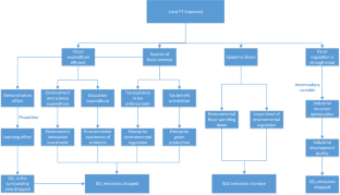
Data availability

Data are obtained from the National Bureau of Statistics, China Statistical Yearbook , and the Research Group of Tsinghua University—Research Report on Financial Transparency of Municipal Governments in China. Ensure availability, authenticity and reliability.

Araujo, J. F. F. E., & Tejedo-Romero, F. (2016). Local government transparency index: Determinants of municipalities’ rankings[J]. International Journal of Public Sector Management, 29 (4), 327–347. https://doi.org/10.1108/IJPSM-11-2015-0199

Article   Google Scholar  

Arbia, G., Battisti, M., & Di Vaio, G. (2010). Institutions and geography: Empirical test of spatial growth models for European regions[J]. Economic Modelling, 27 (1), 12–21. https://doi.org/10.1016/j.econmod.2009.07.004

Bhattacharjee, A., Jensen-Butler, C., (2005). Estimation of spatial weights matrix in a spatial error model, with an application to diffusion in housing demand[J].

Chen, C., Sun, Y., Lan, Q., et al. (2020). Impacts of industrial agglomeration on pollution and ecological efficiency-A spatial econometric analysis based on a big panel dataset of China’s 259 cities[J]. Journal of Cleaner Production, 258 , 120721. https://doi.org/10.1016/j.jclepro.2020.120721

Chen, G., Kang, H., & Luna-Reyes, L. F. (2019). Key determinants of online fiscal transparency: A technology-organization-environment framework[J]. Public Performance & Management Review, 42 (3), 606–631. https://doi.org/10.1080/15309576.2018.1486213

Cole, M. A., Elliott, R. J. R., & Shimamoto, K. (2005). Industrial characteristics, environmental regulations and air pollution: An analysis of the UK manufacturing sector[J]. Journal of Environmental Economics and Management, 50 (1), 121–143. https://doi.org/10.1016/j.jeem.2004.08.001

Dong, F., Wang, Y., Zheng, L., et al. (2020). Can industrial agglomeration promote pollution agglomeration? Evidence from China[J]. Journal of Cleaner Production, 246 , 118960. https://doi.org/10.1016/j.jclepro.2019.118960

Elhorst, J. P. (2014). Matlab software for spatial panels [J]. International Regional Science Review, 37 (3), 389–405. https://doi.org/10.1177/0160017612452429

Feng, Y., Chen, H., Chen, Z., et al. (2021). Has environmental information disclosure eased the economic inhibition of air pollution?[J]. Journal of Cleaner Production, 284 , 125412. https://doi.org/10.1016/j.jclepro.2020.125412

Article   CAS   Google Scholar  

Fingleton, B., & Le Gallo, J. (2008). Estimating spatial models with endogenous variables, a spatial lag and spatially dependent disturbances: Finite sample properties[J]. Papers in Regional Science, 87 (3), 319–339. https://doi.org/10.1111/j.1435-5957.2008.00187.x

Garcia-Murillo, M. (2013). Does a government web presence reduce perceptions of corruption?[J]. Information Technology for Development, 19 (2), 151–175. https://doi.org/10.1080/02681102.2012.751574

Guillamón, M. D., Ríos, A. M., Gesuele, B., et al. (2016). Factors influencing social media use in local governments: The case of Italy and Spain[J]. Government Information Quarterly, 33 (3), 460–471. https://doi.org/10.1016/j.giq.2016.06.005

Hang, Y., Wang, Q., Wang, Y., et al. (2019). Industrial SO 2 emissions treatment in China: A temporal-spatial whole process decomposition analysis[J]. Journal of Environmental Management, 243 , 419–434. https://doi.org/10.1016/j.jenvman.2019.05.025

Heald, D. (2003). Fiscal transparency: Concepts, measurement and UK practice[J]. Public Administration, 81 (4), 723–759. https://doi.org/10.1111/j.0033-3298.2003.00369.x

Li, G., Xue, Q., & Qin, J. (2022). Environmental information disclosure and green technology innovation: Empirical evidence from China[J]. Technological Forecasting and Social Change, 176 , 121453. https://doi.org/10.1016/j.techfore.2021.121453

Li, S. (2014). A differential game of transboundary industrial pollution with emission permits trading[J]. Journal of Optimization Theory and Applications, 163 , 642–659. https://doi.org/10.1007/s10957-013-0384-7

Liu, X., Sun, T., & Feng, Q. (2020). Dynamic spatial spillover effect of urbanization on environmental pollution in China considering the inertia characteristics of environmental pollution[J]. Sustainable Cities and Society, 53 , 101903. https://doi.org/10.1016/j.scs.2019.101903

Lucking-Reiley, D., Bryan, D., Prasad, N., et al. (2007). Pennies from eBay: The determinants of price in online auctions[J]. The Journal of Industrial Economics, 55 (2), 223–233. https://doi.org/10.1111/j.1467-6451.2007.00309.x

Montes, G. C., Bastos, J. C. A., & de Oliveira, A. J. (2019). Fiscal transparency, government effectiveness and government spending efficiency: Some international evidence based on panel data approach[J]. Economic Modelling, 79 , 211–225. https://doi.org/10.1016/j.econmod.2018.10.013

Montes, G. C., & Luna, P. H. (2021). Fiscal transparency, legal system and perception of the control on corruption: Empirical evidence from panel data[J]. Empirical Economics, 60 , 2005–2037. https://doi.org/10.1007/s00181-020-01849-9

Myeong, S., & Shahzad, K. (2021). Integrating data-based strategies and advanced technologies with efficient air pollution management in smart Cities[J]. Sustainability, 13 (13), 7168. https://doi.org/10.3390/su13137168

Qu, J., Zhu, Y. (2019). Government governance, fiscal transparency, and government accounting information sharing: Realization mechanism and path[C]. in: 2019 International Conference on Economic Management and Cultural Industry (ICEMCI 2019) . Atlantis Press, 2019: 806–812. DOI: https://doi.org/10.2991/aebmr.k.191217.143 .

Shen, N., & Peng, H. (2021). Can industrial agglomeration achieve the emission-reduction effect?[J]. Socio-Economic Planning Sciences, 75 , 100867. https://doi.org/10.1016/j.seps.2021.101060

Sinha, A., & Bhattacharya, J. (2017). Estimation of environmental Kuznets curve for SO 2 emission: A case of Indian cities[J]. Ecological Indicators, 72 , 881–894. https://doi.org/10.1016/j.ecolind.2016.02.025

Song, M., Wang, S., Yu, H., et al. (2011). To reduce energy consumption and to maintain rapid economic growth: Analysis of the condition in China based on expended IPAT model[J]. Renewable and Sustainable Energy Reviews, 15 (9), 5129–5134. https://doi.org/10.1016/j.rser.2011.07.043

Wang, E., Su, B., Zhong, S., et al. (2022). China’s Embodied SO 2 Emissions and Aggregate Embodied SO 2 Intensities in Interprovincial and International Trade[J]. Technological Forecasting and Social Change, 177 , 121546. https://doi.org/10.1016/j.techfore.2022.121546

Wang, F., Wei, X., Liu, J., et al. (2019b). Impact of high-speed rail on population mobility and urbanisation: A case study on Yangtze River Delta urban agglomeration, China[J]. Transportation Research Part a: Policy and Practice, 127 , 99–114. https://doi.org/10.1016/j.tra.2019.06.018

Wang, S., & Qiu, J. (2023). The opening of high-speed rail and environmental pollution of the Yangtze River Delta Region in China—based on SDID model test[J]. Environmental Science and Pollution Research, 2023 , 1–10. https://doi.org/10.1007/s11356-023-27439-7

Wang, Y., & He, X. (2019). Spatial economic dependency in the environmental Kuznets Curve of carbon dioxide: The case of China[J]. Journal of Cleaner Production, 218 , 498–510. https://doi.org/10.1016/j.jclepro.2019.01.318

Wang, Z., Li, C., Liu, Q., et al. (2019a). Pollution haven hypothesis of domestic trade in China: A perspective of SO 2 emissions[J]. Science of the Total Environment, 663 , 198–205. https://doi.org/10.1016/j.scitotenv.2019.01.287

Xing, Y., & Brimblecombe, P. (2019). Role of vegetation in deposition and dispersion of air pollution in urban parks[J]. Atmospheric Environment, 201 , 73–83. https://doi.org/10.1016/j.atmosenv.2018.12.027

Xu, C., Zhao, W., Zhang, M., et al. (2021). Pollution haven or halo? The role of the energy transition in the impact of FDI on SO 2 emissions[J]. Science of the Total Environment, 763 , 143002. https://doi.org/10.1016/j.scitotenv.2020.143002

Yang, Q. (2020). Fiscal transparency and public service quality association: Evidence from 12 coastal provinces and cities of China[J]. Journal of Risk and Financial Management, 14 (1), 13. https://doi.org/10.3390/jrfm14010013

Yang, X., Feng, K., Su, B., et al. (2019). Environmental efficiency and equality embodied in China’s inter-regional trade[J]. Science of the Total Environment, 672 , 150–161. https://doi.org/10.1016/j.scitotenv.2019.03.450

Yizhong, W., Ye, H., Qunwei, W., et al. (2021). Cleaner production vs end-of-pipe treatment: Evidence from industrial SO 2 emissions abatement in China[J]. Journal of Environmental Management, 277 , 111429. https://doi.org/10.1016/j.jenvman.2020.111429

Yoro, K. O., & Daramola, M. O. (2020). CO2 emission sources, greenhouse gases, and the global warming effect[M]. Advances in Carbon Capture., 2020 , 3–28. https://doi.org/10.1016/B978-0-12-819657-1.00001-3

Zhang, H., Chen, J., & Wang, Z. (2021). Spatial heterogeneity in spillover effect of air pollution on housing prices: Evidence from China[J]. Cities, 113 , 103145. https://doi.org/10.1016/j.cities.2021.103145

Zhang, Q., Nakatani, J., Shan, Y., et al. (2019). Inter-regional spillover of China’s sulfur dioxide (SO 2 ) pollution across the supply chains[J]. Journal of Cleaner Production, 207 , 418–431. https://doi.org/10.1016/j.jclepro.2018.09.259

Zhang, S., & Wang, L. (2021). The influence of government transparency on governance efficiency in information age: The environmental governance behavior of Guangdong, China[J]. Journal of Enterprise Information Management, 34 (1), 446–459. https://doi.org/10.1108/JEIM-01-2020-0017

Zhao, L., Sun, C., & Liu, F. (2017). Interprovincial two-stage water resource utilization efficiency under environmental constraint and spatial spillover effects in China[J]. Journal of Cleaner Production, 164 , 715–725. https://doi.org/10.1016/j.jclepro.2017.06.252

Zheng, Y., Xue, T., Zhang, Q., et al. (2017). Air quality improvements and health benefits from China’s clean air action since 2013[J]. Environmental Research Letters, 12 (11), 114020. https://doi.org/10.1088/1748-9326/aa8a32

Zhong, S., Li, J., & Zhao, R. (2021). Does environmental information disclosure promote sulfur dioxide (SO 2 ) remove? New evidence from 113 cities in China[J]. Journal of Cleaner Production, 299 , 126906. https://doi.org/10.1016/j.jclepro.2021.126906

Zhu, S., Qiu, X., Yin, Y., et al. (2019). Two-step-hybrid model based on data preprocessing and intelligent optimization algorithms (CS and GWO) for NO2 and SO2 forecasting[J]. Atmospheric Pollution Research, 10 (4), 1326–1335. https://doi.org/10.1016/j.apr.2019.03.004

Download references

We declare that we have no financial and personal relationships with other people or organizations that can inappropriately influence our work, and there is no professional or other personal interest of any nature or kind in any product, service, and/or company that could be construed as influencing the position presented in, or the review of, the manuscript entitled “How does fiscal transparency reduce SO 2 emissions? Treating at the source”.

Author information

Authors and affiliations.

School of Finance and Economics, Harbin Vocational College of Science and Technology, Harbin, Heilongjiang, China

School of Finance, Dongbei University of Finance and Economics, Dalian, Liaoning, China

School of Finance, Harbin University of Commerce, Harbin, Heilongjiang, China

You can also search for this author in PubMed   Google Scholar

Contributions

Yi Qu: Conceptualization, Formal analysis, Writing e review & editing, Resources, Supervision, Project administration. Lang Wang: Methodology, Software, Validation, Formal analysis, Investigation, Data curation, Writing-original draft, Writing-review & editing, Visualization. Shen Zhong: Formal analysis, Writing-original draft, Writing-review & editing.

Corresponding author

Correspondence to Shen Zhong .

Ethics declarations

Conflict of interests.

The authors declare that they have no competing interests.

Consent to publish

All authors agreed to publish.

Additional information

Publisher's note.

Springer Nature remains neutral with regard to jurisdictional claims in published maps and institutional affiliations.

See Figs.  4 and 5 .

Quarterly GDP from 2019 to 2021

Local Moran’I scatter plot based on data of 2011 and 2021

See Table  10 .

Rights and permissions

Springer Nature or its licensor (e.g. a society or other partner) holds exclusive rights to this article under a publishing agreement with the author(s) or other rightsholder(s); author self-archiving of the accepted manuscript version of this article is solely governed by the terms of such publishing agreement and applicable law.

Reprints and permissions

About this article

Qu, Y., Wang, L. & Zhong, S. How does fiscal transparency reduce SO 2 emissions? Treating at the source. Environ Dev Sustain (2024). https://doi.org/10.1007/s10668-024-04769-1

Download citation

Received : 23 November 2022

Accepted : 11 March 2024

Published : 01 April 2024

DOI : https://doi.org/10.1007/s10668-024-04769-1

Share this article

Anyone you share the following link with will be able to read this content:

Sorry, a shareable link is not currently available for this article.

Provided by the Springer Nature SharedIt content-sharing initiative

• Fiscal transparency
• SO 2 emissions
• Environmental governance capacity
• Reverse mediation
• Spatial spillover effect
• Find a journal
• Publish with us
• Track your research

• Commercial Lending
• Community Banking
• Compliance and Risk
• Cybersecurity
• Human Resources
• Mutual Funds
• Retail and Marketing
• Tax and Accounting
• Wealth Management
• Magazine Archive
• Newsletter Archive
• Sponsored Archive
• Podcast Archive

White paper: Financial institutions should refine their cybersecurity amid AI boom

Implementing cutting-edge AI tools to detect and respond to threats is imperative, according to FSSCC. However, it is equally vital to maintain skilled human oversight to interpret AI data accurately and mitigate potential AI inaccuracies or biases, it added. The sector must continue to prioritize the adoption of AI models for fraud prevention, but it also must not forget the human element and prepare for complex phishing and social engineering tactics enabled by AI.

Aligning with approaches like the National Institute of Standards and Technology’s AI Risk Management Framework is critical, according to FSSCC. “Financial institutions must strengthen their risk management protocols, focusing on emerging risks from the increased availability of AI, especially GenAI models, which includes data positioning and model biases,” it said. At the same time, the financial sector should collaborate to develop standardized strategies for managing AI-related risk. Individually, financial institutions should recognize the value of human judgment in AI models and invest in thier workforces.

Regulators also have a role to play, according to FSSCC. “Regulators should identify clear regulatory outcomes and objectives, while enabling regulated entities the ability to deploy effective risk management techniques based on common standards and best practices,” it said.

Related Posts

ABA, state associations urge CFPB to withdraw overdraft proposal

The associations noted that if finalized, the proposal would lead many banks to stop offering—or significantly reduce access to—overdraft, depriving...

Rosenkoetter tapped to lead ABA Card Policy Council 

Thomas Rosenkoetter has been named executive director of the ABA Card Policy Council, which advocates on behalf of the nation’s...

ISM Manufacturing rises in March

U.S. manufacturing activity expanded for the first time in March, following 16 consecutive months of contraction, the Institute for Supply...

Construction spending dropped slightly in February

Construction spending in February was at a seasonally adjusted annual rate of $2.1 trillion, 0.3% below the revised January estimate,...

Federal court pauses CRA rule implementation following ABA lawsuit

A federal judge in Texas issued a preliminary injunction against enforcing new rules implementing the Community Reinvestment Act in a...

Proposed changes delayed to National Flood Insurance Program renewal policies

The Federal Emergency Management Agency recently announced the postponement of the implementation of new guidance regarding the renewal of National...

Two investment advisers agree to pay $400,000 to resolve SEC AI washing allegations

Lender trade groups sue challenging colorado’s ‘rate opt-out law’, new york federal court determines reasonableness of investigation into alleged identity theft is a factual question under fcra, third circuit rules student loan trusts subject to cfpb enforcement authority, virginia district court dismisses foreign currency swap overcharge lawsuit against capital one, sec climate disclosure final rule lawsuit to be heard in 8th circuit, sponsored content.

ERM Model Risk and AI

The Federal Reserve’s Nick Stanescu shares what’s next for the FedNow® Service

AI Compliance and Regulation: What Financial Institutions Need to Know

Gain Efficiencies and Other Timely Benefits with Data Analytics

American Bankers Association 1333 New Hampshire Ave NW Washington, DC 20036 1-800-BANKERS (800-226-5377) www.aba.com About ABA Privacy Policy Contact ABA

© 2024 American Bankers Association. All rights reserved.

Thank you for visiting nature.com. You are using a browser version with limited support for CSS. To obtain the best experience, we recommend you use a more up to date browser (or turn off compatibility mode in Internet Explorer). In the meantime, to ensure continued support, we are displaying the site without styles and JavaScript.

• View all journals
• My Account Login
• Explore content
• About the journal
• Publish with us
• Sign up for alerts
• Open access
• Published: 26 March 2024

Predicting and improving complex beer flavor through machine learning

• Michiel Schreurs   ORCID: orcid.org/0000-0002-9449-5619 1 , 2 , 3   na1 ,
• Supinya Piampongsant 1 , 2 , 3   na1 ,
• Miguel Roncoroni   ORCID: orcid.org/0000-0001-7461-1427 1 , 2 , 3   na1 ,
• Lloyd Cool   ORCID: orcid.org/0000-0001-9936-3124 1 , 2 , 3 , 4 ,
• Beatriz Herrera-Malaver   ORCID: orcid.org/0000-0002-5096-9974 1 , 2 , 3 ,
• Christophe Vanderaa   ORCID: orcid.org/0000-0001-7443-5427 4 ,
• Florian A. Theßeling 1 , 2 , 3 ,
• Łukasz Kreft   ORCID: orcid.org/0000-0001-7620-4657 5 ,
• Alexander Botzki   ORCID: orcid.org/0000-0001-6691-4233 5 ,
• Philippe Malcorps 6 ,
• Luk Daenen 6 ,
• Tom Wenseleers   ORCID: orcid.org/0000-0002-1434-861X 4 &
• Kevin J. Verstrepen   ORCID: orcid.org/0000-0002-3077-6219 1 , 2 , 3  

Nature Communications volume  15 , Article number:  2368 ( 2024 ) Cite this article

41k Accesses

778 Altmetric

Metrics details

• Chemical engineering
• Gas chromatography
• Machine learning
• Metabolomics
• Taste receptors

The perception and appreciation of food flavor depends on many interacting chemical compounds and external factors, and therefore proves challenging to understand and predict. Here, we combine extensive chemical and sensory analyses of 250 different beers to train machine learning models that allow predicting flavor and consumer appreciation. For each beer, we measure over 200 chemical properties, perform quantitative descriptive sensory analysis with a trained tasting panel and map data from over 180,000 consumer reviews to train 10 different machine learning models. The best-performing algorithm, Gradient Boosting, yields models that significantly outperform predictions based on conventional statistics and accurately predict complex food features and consumer appreciation from chemical profiles. Model dissection allows identifying specific and unexpected compounds as drivers of beer flavor and appreciation. Adding these compounds results in variants of commercial alcoholic and non-alcoholic beers with improved consumer appreciation. Together, our study reveals how big data and machine learning uncover complex links between food chemistry, flavor and consumer perception, and lays the foundation to develop novel, tailored foods with superior flavors.

Similar content being viewed by others

BitterSweet: Building machine learning models for predicting the bitter and sweet taste of small molecules

Rudraksh Tuwani, Somin Wadhwa & Ganesh Bagler

Sensory lexicon and aroma volatiles analysis of brewing malt

Xiaoxia Su, Miao Yu, … Tianyi Du

Predicting odor from molecular structure: a multi-label classification approach

Kushagra Saini & Venkatnarayan Ramanathan

Introduction

Predicting and understanding food perception and appreciation is one of the major challenges in food science. Accurate modeling of food flavor and appreciation could yield important opportunities for both producers and consumers, including quality control, product fingerprinting, counterfeit detection, spoilage detection, and the development of new products and product combinations (food pairing) 1 , 2 , 3 , 4 , 5 , 6 . Accurate models for flavor and consumer appreciation would contribute greatly to our scientific understanding of how humans perceive and appreciate flavor. Moreover, accurate predictive models would also facilitate and standardize existing food assessment methods and could supplement or replace assessments by trained and consumer tasting panels, which are variable, expensive and time-consuming 7 , 8 , 9 . Lastly, apart from providing objective, quantitative, accurate and contextual information that can help producers, models can also guide consumers in understanding their personal preferences 10 .

Despite the myriad of applications, predicting food flavor and appreciation from its chemical properties remains a largely elusive goal in sensory science, especially for complex food and beverages 11 , 12 . A key obstacle is the immense number of flavor-active chemicals underlying food flavor. Flavor compounds can vary widely in chemical structure and concentration, making them technically challenging and labor-intensive to quantify, even in the face of innovations in metabolomics, such as non-targeted metabolic fingerprinting 13 , 14 . Moreover, sensory analysis is perhaps even more complicated. Flavor perception is highly complex, resulting from hundreds of different molecules interacting at the physiochemical and sensorial level. Sensory perception is often non-linear, characterized by complex and concentration-dependent synergistic and antagonistic effects 15 , 16 , 17 , 18 , 19 , 20 , 21 that are further convoluted by the genetics, environment, culture and psychology of consumers 22 , 23 , 24 . Perceived flavor is therefore difficult to measure, with problems of sensitivity, accuracy, and reproducibility that can only be resolved by gathering sufficiently large datasets 25 . Trained tasting panels are considered the prime source of quality sensory data, but require meticulous training, are low throughput and high cost. Public databases containing consumer reviews of food products could provide a valuable alternative, especially for studying appreciation scores, which do not require formal training 25 . Public databases offer the advantage of amassing large amounts of data, increasing the statistical power to identify potential drivers of appreciation. However, public datasets suffer from biases, including a bias in the volunteers that contribute to the database, as well as confounding factors such as price, cult status and psychological conformity towards previous ratings of the product.

Classical multivariate statistics and machine learning methods have been used to predict flavor of specific compounds by, for example, linking structural properties of a compound to its potential biological activities or linking concentrations of specific compounds to sensory profiles 1 , 26 . Importantly, most previous studies focused on predicting organoleptic properties of single compounds (often based on their chemical structure) 27 , 28 , 29 , 30 , 31 , 32 , 33 , thus ignoring the fact that these compounds are present in a complex matrix in food or beverages and excluding complex interactions between compounds. Moreover, the classical statistics commonly used in sensory science 34 , 35 , 36 , 37 , 38 , 39 require a large sample size and sufficient variance amongst predictors to create accurate models. They are not fit for studying an extensive set of hundreds of interacting flavor compounds, since they are sensitive to outliers, have a high tendency to overfit and are less suited for non-linear and discontinuous relationships 40 .

In this study, we combine extensive chemical analyses and sensory data of a set of different commercial beers with machine learning approaches to develop models that predict taste, smell, mouthfeel and appreciation from compound concentrations. Beer is particularly suited to model the relationship between chemistry, flavor and appreciation. First, beer is a complex product, consisting of thousands of flavor compounds that partake in complex sensory interactions 41 , 42 , 43 . This chemical diversity arises from the raw materials (malt, yeast, hops, water and spices) and biochemical conversions during the brewing process (kilning, mashing, boiling, fermentation, maturation and aging) 44 , 45 . Second, the advent of the internet saw beer consumers embrace online review platforms, such as RateBeer (ZX Ventures, Anheuser-Busch InBev SA/NV) and BeerAdvocate (Next Glass, inc.). In this way, the beer community provides massive data sets of beer flavor and appreciation scores, creating extraordinarily large sensory databases to complement the analyses of our professional sensory panel. Specifically, we characterize over 200 chemical properties of 250 commercial beers, spread across 22 beer styles, and link these to the descriptive sensory profiling data of a 16-person in-house trained tasting panel and data acquired from over 180,000 public consumer reviews. These unique and extensive datasets enable us to train a suite of machine learning models to predict flavor and appreciation from a beer’s chemical profile. Dissection of the best-performing models allows us to pinpoint specific compounds as potential drivers of beer flavor and appreciation. Follow-up experiments confirm the importance of these compounds and ultimately allow us to significantly improve the flavor and appreciation of selected commercial beers. Together, our study represents a significant step towards understanding complex flavors and reinforces the value of machine learning to develop and refine complex foods. In this way, it represents a stepping stone for further computer-aided food engineering applications 46 .

To generate a comprehensive dataset on beer flavor, we selected 250 commercial Belgian beers across 22 different beer styles (Supplementary Fig.  S1 ). Beers with ≤ 4.2% alcohol by volume (ABV) were classified as non-alcoholic and low-alcoholic. Blonds and Tripels constitute a significant portion of the dataset (12.4% and 11.2%, respectively) reflecting their presence on the Belgian beer market and the heterogeneity of beers within these styles. By contrast, lager beers are less diverse and dominated by a handful of brands. Rare styles such as Brut or Faro make up only a small fraction of the dataset (2% and 1%, respectively) because fewer of these beers are produced and because they are dominated by distinct characteristics in terms of flavor and chemical composition.

Extensive analysis identifies relationships between chemical compounds in beer

For each beer, we measured 226 different chemical properties, including common brewing parameters such as alcohol content, iso-alpha acids, pH, sugar concentration 47 , and over 200 flavor compounds (Methods, Supplementary Table  S1 ). A large portion (37.2%) are terpenoids arising from hopping, responsible for herbal and fruity flavors 16 , 48 . A second major category are yeast metabolites, such as esters and alcohols, that result in fruity and solvent notes 48 , 49 , 50 . Other measured compounds are primarily derived from malt, or other microbes such as non- Saccharomyces yeasts and bacteria (‘wild flora’). Compounds that arise from spices or staling are labeled under ‘Others’. Five attributes (caloric value, total acids and total ester, hop aroma and sulfur compounds) are calculated from multiple individually measured compounds.

As a first step in identifying relationships between chemical properties, we determined correlations between the concentrations of the compounds (Fig.  1 , upper panel, Supplementary Data  1 and 2 , and Supplementary Fig.  S2 . For the sake of clarity, only a subset of the measured compounds is shown in Fig.  1 ). Compounds of the same origin typically show a positive correlation, while absence of correlation hints at parameters varying independently. For example, the hop aroma compounds citronellol, and alpha-terpineol show moderate correlations with each other (Spearman’s rho=0.39 and 0.57), but not with the bittering hop component iso-alpha acids (Spearman’s rho=0.16 and −0.07). This illustrates how brewers can independently modify hop aroma and bitterness by selecting hop varieties and dosage time. If hops are added early in the boiling phase, chemical conversions increase bitterness while aromas evaporate, conversely, late addition of hops preserves aroma but limits bitterness 51 . Similarly, hop-derived iso-alpha acids show a strong anti-correlation with lactic acid and acetic acid, likely reflecting growth inhibition of lactic acid and acetic acid bacteria, or the consequent use of fewer hops in sour beer styles, such as West Flanders ales and Fruit beers, that rely on these bacteria for their distinct flavors 52 . Finally, yeast-derived esters (ethyl acetate, ethyl decanoate, ethyl hexanoate, ethyl octanoate) and alcohols (ethanol, isoamyl alcohol, isobutanol, and glycerol), correlate with Spearman coefficients above 0.5, suggesting that these secondary metabolites are correlated with the yeast genetic background and/or fermentation parameters and may be difficult to influence individually, although the choice of yeast strain may offer some control 53 .

Spearman rank correlations are shown. Descriptors are grouped according to their origin (malt (blue), hops (green), yeast (red), wild flora (yellow), Others (black)), and sensory aspect (aroma, taste, palate, and overall appreciation). Please note that for the chemical compounds, for the sake of clarity, only a subset of the total number of measured compounds is shown, with an emphasis on the key compounds for each source. For more details, see the main text and Methods section. Chemical data can be found in Supplementary Data  1 , correlations between all chemical compounds are depicted in Supplementary Fig.  S2 and correlation values can be found in Supplementary Data  2 . See Supplementary Data  4 for sensory panel assessments and Supplementary Data  5 for correlation values between all sensory descriptors.

Interestingly, different beer styles show distinct patterns for some flavor compounds (Supplementary Fig.  S3 ). These observations agree with expectations for key beer styles, and serve as a control for our measurements. For instance, Stouts generally show high values for color (darker), while hoppy beers contain elevated levels of iso-alpha acids, compounds associated with bitter hop taste. Acetic and lactic acid are not prevalent in most beers, with notable exceptions such as Kriek, Lambic, Faro, West Flanders ales and Flanders Old Brown, which use acid-producing bacteria ( Lactobacillus and Pediococcus ) or unconventional yeast ( Brettanomyces ) 54 , 55 . Glycerol, ethanol and esters show similar distributions across all beer styles, reflecting their common origin as products of yeast metabolism during fermentation 45 , 53 . Finally, low/no-alcohol beers contain low concentrations of glycerol and esters. This is in line with the production process for most of the low/no-alcohol beers in our dataset, which are produced through limiting fermentation or by stripping away alcohol via evaporation or dialysis, with both methods having the unintended side-effect of reducing the amount of flavor compounds in the final beer 56 , 57 .

Besides expected associations, our data also reveals less trivial associations between beer styles and specific parameters. For example, geraniol and citronellol, two monoterpenoids responsible for citrus, floral and rose flavors and characteristic of Citra hops, are found in relatively high amounts in Christmas, Saison, and Brett/co-fermented beers, where they may originate from terpenoid-rich spices such as coriander seeds instead of hops 58 .

Tasting panel assessments reveal sensorial relationships in beer

To assess the sensory profile of each beer, a trained tasting panel evaluated each of the 250 beers for 50 sensory attributes, including different hop, malt and yeast flavors, off-flavors and spices. Panelists used a tasting sheet (Supplementary Data  3 ) to score the different attributes. Panel consistency was evaluated by repeating 12 samples across different sessions and performing ANOVA. In 95% of cases no significant difference was found across sessions ( p  > 0.05), indicating good panel consistency (Supplementary Table  S2 ).

Aroma and taste perception reported by the trained panel are often linked (Fig.  1 , bottom left panel and Supplementary Data  4 and 5 ), with high correlations between hops aroma and taste (Spearman’s rho=0.83). Bitter taste was found to correlate with hop aroma and taste in general (Spearman’s rho=0.80 and 0.69), and particularly with “grassy” noble hops (Spearman’s rho=0.75). Barnyard flavor, most often associated with sour beers, is identified together with stale hops (Spearman’s rho=0.97) that are used in these beers. Lactic and acetic acid, which often co-occur, are correlated (Spearman’s rho=0.66). Interestingly, sweetness and bitterness are anti-correlated (Spearman’s rho = −0.48), confirming the hypothesis that they mask each other 59 , 60 . Beer body is highly correlated with alcohol (Spearman’s rho = 0.79), and overall appreciation is found to correlate with multiple aspects that describe beer mouthfeel (alcohol, carbonation; Spearman’s rho= 0.32, 0.39), as well as with hop and ester aroma intensity (Spearman’s rho=0.39 and 0.35).

Similar to the chemical analyses, sensorial analyses confirmed typical features of specific beer styles (Supplementary Fig.  S4 ). For example, sour beers (Faro, Flanders Old Brown, Fruit beer, Kriek, Lambic, West Flanders ale) were rated acidic, with flavors of both acetic and lactic acid. Hoppy beers were found to be bitter and showed hop-associated aromas like citrus and tropical fruit. Malt taste is most detected among scotch, stout/porters, and strong ales, while low/no-alcohol beers, which often have a reputation for being ‘worty’ (reminiscent of unfermented, sweet malt extract) appear in the middle. Unsurprisingly, hop aromas are most strongly detected among hoppy beers. Like its chemical counterpart (Supplementary Fig.  S3 ), acidity shows a right-skewed distribution, with the most acidic beers being Krieks, Lambics, and West Flanders ales.

Tasting panel assessments of specific flavors correlate with chemical composition

We find that the concentrations of several chemical compounds strongly correlate with specific aroma or taste, as evaluated by the tasting panel (Fig.  2 , Supplementary Fig.  S5 , Supplementary Data  6 ). In some cases, these correlations confirm expectations and serve as a useful control for data quality. For example, iso-alpha acids, the bittering compounds in hops, strongly correlate with bitterness (Spearman’s rho=0.68), while ethanol and glycerol correlate with tasters’ perceptions of alcohol and body, the mouthfeel sensation of fullness (Spearman’s rho=0.82/0.62 and 0.72/0.57 respectively) and darker color from roasted malts is a good indication of malt perception (Spearman’s rho=0.54).

Heatmap colors indicate Spearman’s Rho. Axes are organized according to sensory categories (aroma, taste, mouthfeel, overall), chemical categories and chemical sources in beer (malt (blue), hops (green), yeast (red), wild flora (yellow), Others (black)). See Supplementary Data  6 for all correlation values.

Interestingly, for some relationships between chemical compounds and perceived flavor, correlations are weaker than expected. For example, the rose-smelling phenethyl acetate only weakly correlates with floral aroma. This hints at more complex relationships and interactions between compounds and suggests a need for a more complex model than simple correlations. Lastly, we uncovered unexpected correlations. For instance, the esters ethyl decanoate and ethyl octanoate appear to correlate slightly with hop perception and bitterness, possibly due to their fruity flavor. Iron is anti-correlated with hop aromas and bitterness, most likely because it is also anti-correlated with iso-alpha acids. This could be a sign of metal chelation of hop acids 61 , given that our analyses measure unbound hop acids and total iron content, or could result from the higher iron content in dark and Fruit beers, which typically have less hoppy and bitter flavors 62 .

Public consumer reviews complement expert panel data

To complement and expand the sensory data of our trained tasting panel, we collected 180,000 reviews of our 250 beers from the online consumer review platform RateBeer. This provided numerical scores for beer appearance, aroma, taste, palate, overall quality as well as the average overall score.

Public datasets are known to suffer from biases, such as price, cult status and psychological conformity towards previous ratings of a product. For example, prices correlate with appreciation scores for these online consumer reviews (rho=0.49, Supplementary Fig.  S6 ), but not for our trained tasting panel (rho=0.19). This suggests that prices affect consumer appreciation, which has been reported in wine 63 , while blind tastings are unaffected. Moreover, we observe that some beer styles, like lagers and non-alcoholic beers, generally receive lower scores, reflecting that online reviewers are mostly beer aficionados with a preference for specialty beers over lager beers. In general, we find a modest correlation between our trained panel’s overall appreciation score and the online consumer appreciation scores (Fig.  3 , rho=0.29). Apart from the aforementioned biases in the online datasets, serving temperature, sample freshness and surroundings, which are all tightly controlled during the tasting panel sessions, can vary tremendously across online consumers and can further contribute to (among others, appreciation) differences between the two categories of tasters. Importantly, in contrast to the overall appreciation scores, for many sensory aspects the results from the professional panel correlated well with results obtained from RateBeer reviews. Correlations were highest for features that are relatively easy to recognize even for untrained tasters, like bitterness, sweetness, alcohol and malt aroma (Fig.  3 and below).

RateBeer text mining results can be found in Supplementary Data  7 . Rho values shown are Spearman correlation values, with asterisks indicating significant correlations ( p  < 0.05, two-sided). All p values were smaller than 0.001, except for Esters aroma (0.0553), Esters taste (0.3275), Esters aroma—banana (0.0019), Coriander (0.0508) and Diacetyl (0.0134).

Besides collecting consumer appreciation from these online reviews, we developed automated text analysis tools to gather additional data from review texts (Supplementary Data  7 ). Processing review texts on the RateBeer database yielded comparable results to the scores given by the trained panel for many common sensory aspects, including acidity, bitterness, sweetness, alcohol, malt, and hop tastes (Fig.  3 ). This is in line with what would be expected, since these attributes require less training for accurate assessment and are less influenced by environmental factors such as temperature, serving glass and odors in the environment. Consumer reviews also correlate well with our trained panel for 4-vinyl guaiacol, a compound associated with a very characteristic aroma. By contrast, correlations for more specific aromas like ester, coriander or diacetyl are underrepresented in the online reviews, underscoring the importance of using a trained tasting panel and standardized tasting sheets with explicit factors to be scored for evaluating specific aspects of a beer. Taken together, our results suggest that public reviews are trustworthy for some, but not all, flavor features and can complement or substitute taste panel data for these sensory aspects.

Models can predict beer sensory profiles from chemical data

The rich datasets of chemical analyses, tasting panel assessments and public reviews gathered in the first part of this study provided us with a unique opportunity to develop predictive models that link chemical data to sensorial features. Given the complexity of beer flavor, basic statistical tools such as correlations or linear regression may not always be the most suitable for making accurate predictions. Instead, we applied different machine learning models that can model both simple linear and complex interactive relationships. Specifically, we constructed a set of regression models to predict (a) trained panel scores for beer flavor and quality and (b) public reviews’ appreciation scores from beer chemical profiles. We trained and tested 10 different models (Methods), 3 linear regression-based models (simple linear regression with first-order interactions (LR), lasso regression with first-order interactions (Lasso), partial least squares regressor (PLSR)), 5 decision tree models (AdaBoost regressor (ABR), extra trees (ET), gradient boosting regressor (GBR), random forest (RF) and XGBoost regressor (XGBR)), 1 support vector regression (SVR), and 1 artificial neural network (ANN) model.

To compare the performance of our machine learning models, the dataset was randomly split into a training and test set, stratified by beer style. After a model was trained on data in the training set, its performance was evaluated on its ability to predict the test dataset obtained from multi-output models (based on the coefficient of determination, see Methods). Additionally, individual-attribute models were ranked per descriptor and the average rank was calculated, as proposed by Korneva et al. 64 . Importantly, both ways of evaluating the models’ performance agreed in general. Performance of the different models varied (Table  1 ). It should be noted that all models perform better at predicting RateBeer results than results from our trained tasting panel. One reason could be that sensory data is inherently variable, and this variability is averaged out with the large number of public reviews from RateBeer. Additionally, all tree-based models perform better at predicting taste than aroma. Linear models (LR) performed particularly poorly, with negative R 2 values, due to severe overfitting (training set R 2  = 1). Overfitting is a common issue in linear models with many parameters and limited samples, especially with interaction terms further amplifying the number of parameters. L1 regularization (Lasso) successfully overcomes this overfitting, out-competing multiple tree-based models on the RateBeer dataset. Similarly, the dimensionality reduction of PLSR avoids overfitting and improves performance, to some extent. Still, tree-based models (ABR, ET, GBR, RF and XGBR) show the best performance, out-competing the linear models (LR, Lasso, PLSR) commonly used in sensory science 65 .

GBR models showed the best overall performance in predicting sensory responses from chemical information, with R 2 values up to 0.75 depending on the predicted sensory feature (Supplementary Table  S4 ). The GBR models predict consumer appreciation (RateBeer) better than our trained panel’s appreciation (R 2 value of 0.67 compared to R 2 value of 0.09) (Supplementary Table  S3 and Supplementary Table  S4 ). ANN models showed intermediate performance, likely because neural networks typically perform best with larger datasets 66 . The SVR shows intermediate performance, mostly due to the weak predictions of specific attributes that lower the overall performance (Supplementary Table  S4 ).

Model dissection identifies specific, unexpected compounds as drivers of consumer appreciation

Next, we leveraged our models to infer important contributors to sensory perception and consumer appreciation. Consumer preference is a crucial sensory aspects, because a product that shows low consumer appreciation scores often does not succeed commercially 25 . Additionally, the requirement for a large number of representative evaluators makes consumer trials one of the more costly and time-consuming aspects of product development. Hence, a model for predicting chemical drivers of overall appreciation would be a welcome addition to the available toolbox for food development and optimization.

Since GBR models on our RateBeer dataset showed the best overall performance, we focused on these models. Specifically, we used two approaches to identify important contributors. First, rankings of the most important predictors for each sensorial trait in the GBR models were obtained based on impurity-based feature importance (mean decrease in impurity). High-ranked parameters were hypothesized to be either the true causal chemical properties underlying the trait, to correlate with the actual causal properties, or to take part in sensory interactions affecting the trait 67 (Fig.  4A ). In a second approach, we used SHAP 68 to determine which parameters contributed most to the model for making predictions of consumer appreciation (Fig.  4B ). SHAP calculates parameter contributions to model predictions on a per-sample basis, which can be aggregated into an importance score.

A The impurity-based feature importance (mean deviance in impurity, MDI) calculated from the Gradient Boosting Regression (GBR) model predicting RateBeer appreciation scores. The top 15 highest ranked chemical properties are shown. B SHAP summary plot for the top 15 parameters contributing to our GBR model. Each point on the graph represents a sample from our dataset. The color represents the concentration of that parameter, with bluer colors representing low values and redder colors representing higher values. Greater absolute values on the horizontal axis indicate a higher impact of the parameter on the prediction of the model. C Spearman correlations between the 15 most important chemical properties and consumer overall appreciation. Numbers indicate the Spearman Rho correlation coefficient, and the rank of this correlation compared to all other correlations. The top 15 important compounds were determined using SHAP (panel B).

Both approaches identified ethyl acetate as the most predictive parameter for beer appreciation (Fig.  4 ). Ethyl acetate is the most abundant ester in beer with a typical ‘fruity’, ‘solvent’ and ‘alcoholic’ flavor, but is often considered less important than other esters like isoamyl acetate. The second most important parameter identified by SHAP is ethanol, the most abundant beer compound after water. Apart from directly contributing to beer flavor and mouthfeel, ethanol drastically influences the physical properties of beer, dictating how easily volatile compounds escape the beer matrix to contribute to beer aroma 69 . Importantly, it should also be noted that the importance of ethanol for appreciation is likely inflated by the very low appreciation scores of non-alcoholic beers (Supplementary Fig.  S4 ). Despite not often being considered a driver of beer appreciation, protein level also ranks highly in both approaches, possibly due to its effect on mouthfeel and body 70 . Lactic acid, which contributes to the tart taste of sour beers, is the fourth most important parameter identified by SHAP, possibly due to the generally high appreciation of sour beers in our dataset.

Interestingly, some of the most important predictive parameters for our model are not well-established as beer flavors or are even commonly regarded as being negative for beer quality. For example, our models identify methanethiol and ethyl phenyl acetate, an ester commonly linked to beer staling 71 , as a key factor contributing to beer appreciation. Although there is no doubt that high concentrations of these compounds are considered unpleasant, the positive effects of modest concentrations are not yet known 72 , 73 .

To compare our approach to conventional statistics, we evaluated how well the 15 most important SHAP-derived parameters correlate with consumer appreciation (Fig.  4C ). Interestingly, only 6 of the properties derived by SHAP rank amongst the top 15 most correlated parameters. For some chemical compounds, the correlations are so low that they would have likely been considered unimportant. For example, lactic acid, the fourth most important parameter, shows a bimodal distribution for appreciation, with sour beers forming a separate cluster, that is missed entirely by the Spearman correlation. Additionally, the correlation plots reveal outliers, emphasizing the need for robust analysis tools. Together, this highlights the need for alternative models, like the Gradient Boosting model, that better grasp the complexity of (beer) flavor.

Finally, to observe the relationships between these chemical properties and their predicted targets, partial dependence plots were constructed for the six most important predictors of consumer appreciation 74 , 75 , 76 (Supplementary Fig.  S7 ). One-way partial dependence plots show how a change in concentration affects the predicted appreciation. These plots reveal an important limitation of our models: appreciation predictions remain constant at ever-increasing concentrations. This implies that once a threshold concentration is reached, further increasing the concentration does not affect appreciation. This is false, as it is well-documented that certain compounds become unpleasant at high concentrations, including ethyl acetate (‘nail polish’) 77 and methanethiol (‘sulfury’ and ‘rotten cabbage’) 78 . The inability of our models to grasp that flavor compounds have optimal levels, above which they become negative, is a consequence of working with commercial beer brands where (off-)flavors are rarely too high to negatively impact the product. The two-way partial dependence plots show how changing the concentration of two compounds influences predicted appreciation, visualizing their interactions (Supplementary Fig.  S7 ). In our case, the top 5 parameters are dominated by additive or synergistic interactions, with high concentrations for both compounds resulting in the highest predicted appreciation.

To assess the robustness of our best-performing models and model predictions, we performed 100 iterations of the GBR, RF and ET models. In general, all iterations of the models yielded similar performance (Supplementary Fig.  S8 ). Moreover, the main predictors (including the top predictors ethanol and ethyl acetate) remained virtually the same, especially for GBR and RF. For the iterations of the ET model, we did observe more variation in the top predictors, which is likely a consequence of the model’s inherent random architecture in combination with co-correlations between certain predictors. However, even in this case, several of the top predictors (ethanol and ethyl acetate) remain unchanged, although their rank in importance changes (Supplementary Fig.  S8 ).

Next, we investigated if a combination of RateBeer and trained panel data into one consolidated dataset would lead to stronger models, under the hypothesis that such a model would suffer less from bias in the datasets. A GBR model was trained to predict appreciation on the combined dataset. This model underperformed compared to the RateBeer model, both in the native case and when including a dataset identifier (R 2  = 0.67, 0.26 and 0.42 respectively). For the latter, the dataset identifier is the most important feature (Supplementary Fig.  S9 ), while most of the feature importance remains unchanged, with ethyl acetate and ethanol ranking highest, like in the original model trained only on RateBeer data. It seems that the large variation in the panel dataset introduces noise, weakening the models’ performances and reliability. In addition, it seems reasonable to assume that both datasets are fundamentally different, with the panel dataset obtained by blind tastings by a trained professional panel.

Lastly, we evaluated whether beer style identifiers would further enhance the model’s performance. A GBR model was trained with parameters that explicitly encoded the styles of the samples. This did not improve model performance (R2 = 0.66 with style information vs R2 = 0.67). The most important chemical features are consistent with the model trained without style information (eg. ethanol and ethyl acetate), and with the exception of the most preferred (strong ale) and least preferred (low/no-alcohol) styles, none of the styles were among the most important features (Supplementary Fig.  S9 , Supplementary Table  S5 and S6 ). This is likely due to a combination of style-specific chemical signatures, such as iso-alpha acids and lactic acid, that implicitly convey style information to the original models, as well as the low number of samples belonging to some styles, making it difficult for the model to learn style-specific patterns. Moreover, beer styles are not rigorously defined, with some styles overlapping in features and some beers being misattributed to a specific style, all of which leads to more noise in models that use style parameters.

Model validation

To test if our predictive models give insight into beer appreciation, we set up experiments aimed at improving existing commercial beers. We specifically selected overall appreciation as the trait to be examined because of its complexity and commercial relevance. Beer flavor comprises a complex bouquet rather than single aromas and tastes 53 . Hence, adding a single compound to the extent that a difference is noticeable may lead to an unbalanced, artificial flavor. Therefore, we evaluated the effect of combinations of compounds. Because Blond beers represent the most extensive style in our dataset, we selected a beer from this style as the starting material for these experiments (Beer 64 in Supplementary Data  1 ).

In the first set of experiments, we adjusted the concentrations of compounds that made up the most important predictors of overall appreciation (ethyl acetate, ethanol, lactic acid, ethyl phenyl acetate) together with correlated compounds (ethyl hexanoate, isoamyl acetate, glycerol), bringing them up to 95 th percentile ethanol-normalized concentrations (Methods) within the Blond group (‘Spiked’ concentration in Fig.  5A ). Compared to controls, the spiked beers were found to have significantly improved overall appreciation among trained panelists, with panelist noting increased intensity of ester flavors, sweetness, alcohol, and body fullness (Fig.  5B ). To disentangle the contribution of ethanol to these results, a second experiment was performed without the addition of ethanol. This resulted in a similar outcome, including increased perception of alcohol and overall appreciation.

Adding the top chemical compounds, identified as best predictors of appreciation by our model, into poorly appreciated beers results in increased appreciation from our trained panel. Results of sensory tests between base beers and those spiked with compounds identified as the best predictors by the model. A Blond and Non/Low-alcohol (0.0% ABV) base beers were brought up to 95th-percentile ethanol-normalized concentrations within each style. B For each sensory attribute, tasters indicated the more intense sample and selected the sample they preferred. The numbers above the bars correspond to the p values that indicate significant changes in perceived flavor (two-sided binomial test: alpha 0.05, n  = 20 or 13).

In a last experiment, we tested whether using the model’s predictions can boost the appreciation of a non-alcoholic beer (beer 223 in Supplementary Data  1 ). Again, the addition of a mixture of predicted compounds (omitting ethanol, in this case) resulted in a significant increase in appreciation, body, ester flavor and sweetness.

Predicting flavor and consumer appreciation from chemical composition is one of the ultimate goals of sensory science. A reliable, systematic and unbiased way to link chemical profiles to flavor and food appreciation would be a significant asset to the food and beverage industry. Such tools would substantially aid in quality control and recipe development, offer an efficient and cost-effective alternative to pilot studies and consumer trials and would ultimately allow food manufacturers to produce superior, tailor-made products that better meet the demands of specific consumer groups more efficiently.

A limited set of studies have previously tried, to varying degrees of success, to predict beer flavor and beer popularity based on (a limited set of) chemical compounds and flavors 79 , 80 . Current sensitive, high-throughput technologies allow measuring an unprecedented number of chemical compounds and properties in a large set of samples, yielding a dataset that can train models that help close the gaps between chemistry and flavor, even for a complex natural product like beer. To our knowledge, no previous research gathered data at this scale (250 samples, 226 chemical parameters, 50 sensory attributes and 5 consumer scores) to disentangle and validate the chemical aspects driving beer preference using various machine-learning techniques. We find that modern machine learning models outperform conventional statistical tools, such as correlations and linear models, and can successfully predict flavor appreciation from chemical composition. This could be attributed to the natural incorporation of interactions and non-linear or discontinuous effects in machine learning models, which are not easily grasped by the linear model architecture. While linear models and partial least squares regression represent the most widespread statistical approaches in sensory science, in part because they allow interpretation 65 , 81 , 82 , modern machine learning methods allow for building better predictive models while preserving the possibility to dissect and exploit the underlying patterns. Of the 10 different models we trained, tree-based models, such as our best performing GBR, showed the best overall performance in predicting sensory responses from chemical information, outcompeting artificial neural networks. This agrees with previous reports for models trained on tabular data 83 . Our results are in line with the findings of Colantonio et al. who also identified the gradient boosting architecture as performing best at predicting appreciation and flavor (of tomatoes and blueberries, in their specific study) 26 . Importantly, besides our larger experimental scale, we were able to directly confirm our models’ predictions in vivo.

Our study confirms that flavor compound concentration does not always correlate with perception, suggesting complex interactions that are often missed by more conventional statistics and simple models. Specifically, we find that tree-based algorithms may perform best in developing models that link complex food chemistry with aroma. Furthermore, we show that massive datasets of untrained consumer reviews provide a valuable source of data, that can complement or even replace trained tasting panels, especially for appreciation and basic flavors, such as sweetness and bitterness. This holds despite biases that are known to occur in such datasets, such as price or conformity bias. Moreover, GBR models predict taste better than aroma. This is likely because taste (e.g. bitterness) often directly relates to the corresponding chemical measurements (e.g., iso-alpha acids), whereas such a link is less clear for aromas, which often result from the interplay between multiple volatile compounds. We also find that our models are best at predicting acidity and alcohol, likely because there is a direct relation between the measured chemical compounds (acids and ethanol) and the corresponding perceived sensorial attribute (acidity and alcohol), and because even untrained consumers are generally able to recognize these flavors and aromas.

The predictions of our final models, trained on review data, hold even for blind tastings with small groups of trained tasters, as demonstrated by our ability to validate specific compounds as drivers of beer flavor and appreciation. Since adding a single compound to the extent of a noticeable difference may result in an unbalanced flavor profile, we specifically tested our identified key drivers as a combination of compounds. While this approach does not allow us to validate if a particular single compound would affect flavor and/or appreciation, our experiments do show that this combination of compounds increases consumer appreciation.

It is important to stress that, while it represents an important step forward, our approach still has several major limitations. A key weakness of the GBR model architecture is that amongst co-correlating variables, the largest main effect is consistently preferred for model building. As a result, co-correlating variables often have artificially low importance scores, both for impurity and SHAP-based methods, like we observed in the comparison to the more randomized Extra Trees models. This implies that chemicals identified as key drivers of a specific sensory feature by GBR might not be the true causative compounds, but rather co-correlate with the actual causative chemical. For example, the high importance of ethyl acetate could be (partially) attributed to the total ester content, ethanol or ethyl hexanoate (rho=0.77, rho=0.72 and rho=0.68), while ethyl phenylacetate could hide the importance of prenyl isobutyrate and ethyl benzoate (rho=0.77 and rho=0.76). Expanding our GBR model to include beer style as a parameter did not yield additional power or insight. This is likely due to style-specific chemical signatures, such as iso-alpha acids and lactic acid, that implicitly convey style information to the original model, as well as the smaller sample size per style, limiting the power to uncover style-specific patterns. This can be partly attributed to the curse of dimensionality, where the high number of parameters results in the models mainly incorporating single parameter effects, rather than complex interactions such as style-dependent effects 67 . A larger number of samples may overcome some of these limitations and offer more insight into style-specific effects. On the other hand, beer style is not a rigid scientific classification, and beers within one style often differ a lot, which further complicates the analysis of style as a model factor.

Our study is limited to beers from Belgian breweries. Although these beers cover a large portion of the beer styles available globally, some beer styles and consumer patterns may be missing, while other features might be overrepresented. For example, many Belgian ales exhibit yeast-driven flavor profiles, which is reflected in the chemical drivers of appreciation discovered by this study. In future work, expanding the scope to include diverse markets and beer styles could lead to the identification of even more drivers of appreciation and better models for special niche products that were not present in our beer set.

In addition to inherent limitations of GBR models, there are also some limitations associated with studying food aroma. Even if our chemical analyses measured most of the known aroma compounds, the total number of flavor compounds in complex foods like beer is still larger than the subset we were able to measure in this study. For example, hop-derived thiols, that influence flavor at very low concentrations, are notoriously difficult to measure in a high-throughput experiment. Moreover, consumer perception remains subjective and prone to biases that are difficult to avoid. It is also important to stress that the models are still immature and that more extensive datasets will be crucial for developing more complete models in the future. Besides more samples and parameters, our dataset does not include any demographic information about the tasters. Including such data could lead to better models that grasp external factors like age and culture. Another limitation is that our set of beers consists of high-quality end-products and lacks beers that are unfit for sale, which limits the current model in accurately predicting products that are appreciated very badly. Finally, while models could be readily applied in quality control, their use in sensory science and product development is restrained by their inability to discern causal relationships. Given that the models cannot distinguish compounds that genuinely drive consumer perception from those that merely correlate, validation experiments are essential to identify true causative compounds.

Despite the inherent limitations, dissection of our models enabled us to pinpoint specific molecules as potential drivers of beer aroma and consumer appreciation, including compounds that were unexpected and would not have been identified using standard approaches. Important drivers of beer appreciation uncovered by our models include protein levels, ethyl acetate, ethyl phenyl acetate and lactic acid. Currently, many brewers already use lactic acid to acidify their brewing water and ensure optimal pH for enzymatic activity during the mashing process. Our results suggest that adding lactic acid can also improve beer appreciation, although its individual effect remains to be tested. Interestingly, ethanol appears to be unnecessary to improve beer appreciation, both for blond beer and alcohol-free beer. Given the growing consumer interest in alcohol-free beer, with a predicted annual market growth of >7% 84 , it is relevant for brewers to know what compounds can further increase consumer appreciation of these beers. Hence, our model may readily provide avenues to further improve the flavor and consumer appreciation of both alcoholic and non-alcoholic beers, which is generally considered one of the key challenges for future beer production.

Whereas we see a direct implementation of our results for the development of superior alcohol-free beverages and other food products, our study can also serve as a stepping stone for the development of novel alcohol-containing beverages. We want to echo the growing body of scientific evidence for the negative effects of alcohol consumption, both on the individual level by the mutagenic, teratogenic and carcinogenic effects of ethanol 85 , 86 , as well as the burden on society caused by alcohol abuse and addiction. We encourage the use of our results for the production of healthier, tastier products, including novel and improved beverages with lower alcohol contents. Furthermore, we strongly discourage the use of these technologies to improve the appreciation or addictive properties of harmful substances.

The present work demonstrates that despite some important remaining hurdles, combining the latest developments in chemical analyses, sensory analysis and modern machine learning methods offers exciting avenues for food chemistry and engineering. Soon, these tools may provide solutions in quality control and recipe development, as well as new approaches to sensory science and flavor research.

Beer selection

250 commercial Belgian beers were selected to cover the broad diversity of beer styles and corresponding diversity in chemical composition and aroma. See Supplementary Fig.  S1 .

Chemical dataset

Sample preparation.

Beers within their expiration date were purchased from commercial retailers. Samples were prepared in biological duplicates at room temperature, unless explicitly stated otherwise. Bottle pressure was measured with a manual pressure device (Steinfurth Mess-Systeme GmbH) and used to calculate CO 2 concentration. The beer was poured through two filter papers (Macherey-Nagel, 500713032 MN 713 ¼) to remove carbon dioxide and prevent spontaneous foaming. Samples were then prepared for measurements by targeted Headspace-Gas Chromatography-Flame Ionization Detector/Flame Photometric Detector (HS-GC-FID/FPD), Headspace-Solid Phase Microextraction-Gas Chromatography-Mass Spectrometry (HS-SPME-GC-MS), colorimetric analysis, enzymatic analysis, Near-Infrared (NIR) analysis, as described in the sections below. The mean values of biological duplicates are reported for each compound.

HS-GC-FID/FPD

HS-GC-FID/FPD (Shimadzu GC 2010 Plus) was used to measure higher alcohols, acetaldehyde, esters, 4-vinyl guaicol, and sulfur compounds. Each measurement comprised 5 ml of sample pipetted into a 20 ml glass vial containing 1.75 g NaCl (VWR, 27810.295). 100 µl of 2-heptanol (Sigma-Aldrich, H3003) (internal standard) solution in ethanol (Fisher Chemical, E/0650DF/C17) was added for a final concentration of 2.44 mg/L. Samples were flushed with nitrogen for 10 s, sealed with a silicone septum, stored at −80 °C and analyzed in batches of 20.

The GC was equipped with a DB-WAXetr column (length, 30 m; internal diameter, 0.32 mm; layer thickness, 0.50 µm; Agilent Technologies, Santa Clara, CA, USA) to the FID and an HP-5 column (length, 30 m; internal diameter, 0.25 mm; layer thickness, 0.25 µm; Agilent Technologies, Santa Clara, CA, USA) to the FPD. N 2 was used as the carrier gas. Samples were incubated for 20 min at 70 °C in the headspace autosampler (Flow rate, 35 cm/s; Injection volume, 1000 µL; Injection mode, split; Combi PAL autosampler, CTC analytics, Switzerland). The injector, FID and FPD temperatures were kept at 250 °C. The GC oven temperature was first held at 50 °C for 5 min and then allowed to rise to 80 °C at a rate of 5 °C/min, followed by a second ramp of 4 °C/min until 200 °C kept for 3 min and a final ramp of (4 °C/min) until 230 °C for 1 min. Results were analyzed with the GCSolution software version 2.4 (Shimadzu, Kyoto, Japan). The GC was calibrated with a 5% EtOH solution (VWR International) containing the volatiles under study (Supplementary Table  S7 ).

HS-SPME-GC-MS

HS-SPME-GC-MS (Shimadzu GCMS-QP-2010 Ultra) was used to measure additional volatile compounds, mainly comprising terpenoids and esters. Samples were analyzed by HS-SPME using a triphase DVB/Carboxen/PDMS 50/30 μm SPME fiber (Supelco Co., Bellefonte, PA, USA) followed by gas chromatography (Thermo Fisher Scientific Trace 1300 series, USA) coupled to a mass spectrometer (Thermo Fisher Scientific ISQ series MS) equipped with a TriPlus RSH autosampler. 5 ml of degassed beer sample was placed in 20 ml vials containing 1.75 g NaCl (VWR, 27810.295). 5 µl internal standard mix was added, containing 2-heptanol (1 g/L) (Sigma-Aldrich, H3003), 4-fluorobenzaldehyde (1 g/L) (Sigma-Aldrich, 128376), 2,3-hexanedione (1 g/L) (Sigma-Aldrich, 144169) and guaiacol (1 g/L) (Sigma-Aldrich, W253200) in ethanol (Fisher Chemical, E/0650DF/C17). Each sample was incubated at 60 °C in the autosampler oven with constant agitation. After 5 min equilibration, the SPME fiber was exposed to the sample headspace for 30 min. The compounds trapped on the fiber were thermally desorbed in the injection port of the chromatograph by heating the fiber for 15 min at 270 °C.

The GC-MS was equipped with a low polarity RXi-5Sil MS column (length, 20 m; internal diameter, 0.18 mm; layer thickness, 0.18 µm; Restek, Bellefonte, PA, USA). Injection was performed in splitless mode at 320 °C, a split flow of 9 ml/min, a purge flow of 5 ml/min and an open valve time of 3 min. To obtain a pulsed injection, a programmed gas flow was used whereby the helium gas flow was set at 2.7 mL/min for 0.1 min, followed by a decrease in flow of 20 ml/min to the normal 0.9 mL/min. The temperature was first held at 30 °C for 3 min and then allowed to rise to 80 °C at a rate of 7 °C/min, followed by a second ramp of 2 °C/min till 125 °C and a final ramp of 8 °C/min with a final temperature of 270 °C.

Mass acquisition range was 33 to 550 amu at a scan rate of 5 scans/s. Electron impact ionization energy was 70 eV. The interface and ion source were kept at 275 °C and 250 °C, respectively. A mix of linear n-alkanes (from C7 to C40, Supelco Co.) was injected into the GC-MS under identical conditions to serve as external retention index markers. Identification and quantification of the compounds were performed using an in-house developed R script as described in Goelen et al. and Reher et al. 87 , 88 (for package information, see Supplementary Table  S8 ). Briefly, chromatograms were analyzed using AMDIS (v2.71) 89 to separate overlapping peaks and obtain pure compound spectra. The NIST MS Search software (v2.0 g) in combination with the NIST2017, FFNSC3 and Adams4 libraries were used to manually identify the empirical spectra, taking into account the expected retention time. After background subtraction and correcting for retention time shifts between samples run on different days based on alkane ladders, compound elution profiles were extracted and integrated using a file with 284 target compounds of interest, which were either recovered in our identified AMDIS list of spectra or were known to occur in beer. Compound elution profiles were estimated for every peak in every chromatogram over a time-restricted window using weighted non-negative least square analysis after which peak areas were integrated 87 , 88 . Batch effect correction was performed by normalizing against the most stable internal standard compound, 4-fluorobenzaldehyde. Out of all 284 target compounds that were analyzed, 167 were visually judged to have reliable elution profiles and were used for final analysis.

Discrete photometric and enzymatic analysis

Discrete photometric and enzymatic analysis (Thermo Scientific TM Gallery TM Plus Beermaster Discrete Analyzer) was used to measure acetic acid, ammonia, beta-glucan, iso-alpha acids, color, sugars, glycerol, iron, pH, protein, and sulfite. 2 ml of sample volume was used for the analyses. Information regarding the reagents and standard solutions used for analyses and calibrations is included in Supplementary Table  S7 and Supplementary Table  S9 .

NIR analyses

NIR analysis (Anton Paar Alcolyzer Beer ME System) was used to measure ethanol. Measurements comprised 50 ml of sample, and a 10% EtOH solution was used for calibration.

Correlation calculations

Pairwise Spearman Rank correlations were calculated between all chemical properties.

Sensory dataset

Trained panel.

Our trained tasting panel consisted of volunteers who gave prior verbal informed consent. All compounds used for the validation experiment were of food-grade quality. The tasting sessions were approved by the Social and Societal Ethics Committee of the KU Leuven (G-2022-5677-R2(MAR)). All online reviewers agreed to the Terms and Conditions of the RateBeer website.

Sensory analysis was performed according to the American Society of Brewing Chemists (ASBC) Sensory Analysis Methods 90 . 30 volunteers were screened through a series of triangle tests. The sixteen most sensitive and consistent tasters were retained as taste panel members. The resulting panel was diverse in age [22–42, mean: 29], sex [56% male] and nationality [7 different countries]. The panel developed a consensus vocabulary to describe beer aroma, taste and mouthfeel. Panelists were trained to identify and score 50 different attributes, using a 7-point scale to rate attributes’ intensity. The scoring sheet is included as Supplementary Data  3 . Sensory assessments took place between 10–12 a.m. The beers were served in black-colored glasses. Per session, between 5 and 12 beers of the same style were tasted at 12 °C to 16 °C. Two reference beers were added to each set and indicated as ‘Reference 1 & 2’, allowing panel members to calibrate their ratings. Not all panelists were present at every tasting. Scores were scaled by standard deviation and mean-centered per taster. Values are represented as z-scores and clustered by Euclidean distance. Pairwise Spearman correlations were calculated between taste and aroma sensory attributes. Panel consistency was evaluated by repeating samples on different sessions and performing ANOVA to identify differences, using the ‘stats’ package (v4.2.2) in R (for package information, see Supplementary Table  S8 ).

Online reviews from a public database

The ‘scrapy’ package in Python (v3.6) (for package information, see Supplementary Table  S8 ). was used to collect 232,288 online reviews (mean=922, min=6, max=5343) from RateBeer, an online beer review database. Each review entry comprised 5 numerical scores (appearance, aroma, taste, palate and overall quality) and an optional review text. The total number of reviews per reviewer was collected separately. Numerical scores were scaled and centered per rater, and mean scores were calculated per beer.

For the review texts, the language was estimated using the packages ‘langdetect’ and ‘langid’ in Python. Reviews that were classified as English by both packages were kept. Reviewers with fewer than 100 entries overall were discarded. 181,025 reviews from >6000 reviewers from >40 countries remained. Text processing was done using the ‘nltk’ package in Python. Texts were corrected for slang and misspellings; proper nouns and rare words that are relevant to the beer context were specified and kept as-is (‘Chimay’,’Lambic’, etc.). A dictionary of semantically similar sensorial terms, for example ‘floral’ and ‘flower’, was created and collapsed together into one term. Words were stemmed and lemmatized to avoid identifying words such as ‘acid’ and ‘acidity’ as separate terms. Numbers and punctuation were removed.

Sentences from up to 50 randomly chosen reviews per beer were manually categorized according to the aspect of beer they describe (appearance, aroma, taste, palate, overall quality—not to be confused with the 5 numerical scores described above) or flagged as irrelevant if they contained no useful information. If a beer contained fewer than 50 reviews, all reviews were manually classified. This labeled data set was used to train a model that classified the rest of the sentences for all beers 91 . Sentences describing taste and aroma were extracted, and term frequency–inverse document frequency (TFIDF) was implemented to calculate enrichment scores for sensorial words per beer.

The sex of the tasting subject was not considered when building our sensory database. Instead, results from different panelists were averaged, both for our trained panel (56% male, 44% female) and the RateBeer reviews (70% male, 30% female for RateBeer as a whole).

Beer price collection and processing

Beer prices were collected from the following stores: Colruyt, Delhaize, Total Wine, BeerHawk, The Belgian Beer Shop, The Belgian Shop, and Beer of Belgium. Where applicable, prices were converted to Euros and normalized per liter. Spearman correlations were calculated between these prices and mean overall appreciation scores from RateBeer and the taste panel, respectively.

Pairwise Spearman Rank correlations were calculated between all sensory properties.

Machine learning models

Predictive modeling of sensory profiles from chemical data.

Regression models were constructed to predict (a) trained panel scores for beer flavors and quality from beer chemical profiles and (b) public reviews’ appreciation scores from beer chemical profiles. Z-scores were used to represent sensory attributes in both data sets. Chemical properties with log-normal distributions (Shapiro-Wilk test, p  <  0.05 ) were log-transformed. Missing chemical measurements (0.1% of all data) were replaced with mean values per attribute. Observations from 250 beers were randomly separated into a training set (70%, 175 beers) and a test set (30%, 75 beers), stratified per beer style. Chemical measurements (p = 231) were normalized based on the training set average and standard deviation. In total, three linear regression-based models: linear regression with first-order interaction terms (LR), lasso regression with first-order interaction terms (Lasso) and partial least squares regression (PLSR); five decision tree models, Adaboost regressor (ABR), Extra Trees (ET), Gradient Boosting regressor (GBR), Random Forest (RF) and XGBoost regressor (XGBR); one support vector machine model (SVR) and one artificial neural network model (ANN) were trained. The models were implemented using the ‘scikit-learn’ package (v1.2.2) and ‘xgboost’ package (v1.7.3) in Python (v3.9.16). Models were trained, and hyperparameters optimized, using five-fold cross-validated grid search with the coefficient of determination (R 2 ) as the evaluation metric. The ANN (scikit-learn’s MLPRegressor) was optimized using Bayesian Tree-Structured Parzen Estimator optimization with the ‘Optuna’ Python package (v3.2.0). Individual models were trained per attribute, and a multi-output model was trained on all attributes simultaneously.

Model dissection

GBR was found to outperform other methods, resulting in models with the highest average R 2 values in both trained panel and public review data sets. Impurity-based rankings of the most important predictors for each predicted sensorial trait were obtained using the ‘scikit-learn’ package. To observe the relationships between these chemical properties and their predicted targets, partial dependence plots (PDP) were constructed for the six most important predictors of consumer appreciation 74 , 75 .

The ‘SHAP’ package in Python (v0.41.0) was implemented to provide an alternative ranking of predictor importance and to visualize the predictors’ effects as a function of their concentration 68 .

Validation of causal chemical properties

To validate the effects of the most important model features on predicted sensory attributes, beers were spiked with the chemical compounds identified by the models and descriptive sensory analyses were carried out according to the American Society of Brewing Chemists (ASBC) protocol 90 .

Compound spiking was done 30 min before tasting. Compounds were spiked into fresh beer bottles, that were immediately resealed and inverted three times. Fresh bottles of beer were opened for the same duration, resealed, and inverted thrice, to serve as controls. Pairs of spiked samples and controls were served simultaneously, chilled and in dark glasses as outlined in the Trained panel section above. Tasters were instructed to select the glass with the higher flavor intensity for each attribute (directional difference test 92 ) and to select the glass they prefer.

The final concentration after spiking was equal to the within-style average, after normalizing by ethanol concentration. This was done to ensure balanced flavor profiles in the final spiked beer. The same methods were applied to improve a non-alcoholic beer. Compounds were the following: ethyl acetate (Merck KGaA, W241415), ethyl hexanoate (Merck KGaA, W243906), isoamyl acetate (Merck KGaA, W205508), phenethyl acetate (Merck KGaA, W285706), ethanol (96%, Colruyt), glycerol (Merck KGaA, W252506), lactic acid (Merck KGaA, 261106).

Significant differences in preference or perceived intensity were determined by performing the two-sided binomial test on each attribute.

Reporting summary

Further information on research design is available in the  Nature Portfolio Reporting Summary linked to this article.

Data availability

The data that support the findings of this work are available in the Supplementary Data files and have been deposited to Zenodo under accession code 10653704 93 . The RateBeer scores data are under restricted access, they are not publicly available as they are property of RateBeer (ZX Ventures, USA). Access can be obtained from the authors upon reasonable request and with permission of RateBeer (ZX Ventures, USA).  Source data are provided with this paper.

Code availability

The code for training the machine learning models, analyzing the models, and generating the figures has been deposited to Zenodo under accession code 10653704 93 .

Tieman, D. et al. A chemical genetic roadmap to improved tomato flavor. Science 355 , 391–394 (2017).

Article   ADS   CAS   PubMed   Google Scholar  

Plutowska, B. & Wardencki, W. Application of gas chromatography–olfactometry (GC–O) in analysis and quality assessment of alcoholic beverages – A review. Food Chem. 107 , 449–463 (2008).

Article   CAS   Google Scholar  

Legin, A., Rudnitskaya, A., Seleznev, B. & Vlasov, Y. Electronic tongue for quality assessment of ethanol, vodka and eau-de-vie. Anal. Chim. Acta 534 , 129–135 (2005).

Loutfi, A., Coradeschi, S., Mani, G. K., Shankar, P. & Rayappan, J. B. B. Electronic noses for food quality: A review. J. Food Eng. 144 , 103–111 (2015).

Ahn, Y.-Y., Ahnert, S. E., Bagrow, J. P. & Barabási, A.-L. Flavor network and the principles of food pairing. Sci. Rep. 1 , 196 (2011).

Article   CAS   PubMed   PubMed Central   Google Scholar  

Bartoshuk, L. M. & Klee, H. J. Better fruits and vegetables through sensory analysis. Curr. Biol. 23 , R374–R378 (2013).

Article   CAS   PubMed   Google Scholar  

Piggott, J. R. Design questions in sensory and consumer science. Food Qual. Prefer. 3293 , 217–220 (1995).

Article   Google Scholar  

Kermit, M. & Lengard, V. Assessing the performance of a sensory panel-panellist monitoring and tracking. J. Chemom. 19 , 154–161 (2005).

Cook, D. J., Hollowood, T. A., Linforth, R. S. T. & Taylor, A. J. Correlating instrumental measurements of texture and flavour release with human perception. Int. J. Food Sci. Technol. 40 , 631–641 (2005).

Chinchanachokchai, S., Thontirawong, P. & Chinchanachokchai, P. A tale of two recommender systems: The moderating role of consumer expertise on artificial intelligence based product recommendations. J. Retail. Consum. Serv. 61 , 1–12 (2021).

Ross, C. F. Sensory science at the human-machine interface. Trends Food Sci. Technol. 20 , 63–72 (2009).

Chambers, E. IV & Koppel, K. Associations of volatile compounds with sensory aroma and flavor: The complex nature of flavor. Molecules 18 , 4887–4905 (2013).

Pinu, F. R. Metabolomics—The new frontier in food safety and quality research. Food Res. Int. 72 , 80–81 (2015).

Danezis, G. P., Tsagkaris, A. S., Brusic, V. & Georgiou, C. A. Food authentication: state of the art and prospects. Curr. Opin. Food Sci. 10 , 22–31 (2016).

Shepherd, G. M. Smell images and the flavour system in the human brain. Nature 444 , 316–321 (2006).

Meilgaard, M. C. Prediction of flavor differences between beers from their chemical composition. J. Agric. Food Chem. 30 , 1009–1017 (1982).

Xu, L. et al. Widespread receptor-driven modulation in peripheral olfactory coding. Science 368 , eaaz5390 (2020).

Kupferschmidt, K. Following the flavor. Science 340 , 808–809 (2013).

Billesbølle, C. B. et al. Structural basis of odorant recognition by a human odorant receptor. Nature 615 , 742–749 (2023).

Article   ADS   PubMed   PubMed Central   Google Scholar  

Smith, B. Perspective: Complexities of flavour. Nature 486 , S6–S6 (2012).

Pfister, P. et al. Odorant receptor inhibition is fundamental to odor encoding. Curr. Biol. 30 , 2574–2587 (2020).

Moskowitz, H. W., Kumaraiah, V., Sharma, K. N., Jacobs, H. L. & Sharma, S. D. Cross-cultural differences in simple taste preferences. Science 190 , 1217–1218 (1975).

Eriksson, N. et al. A genetic variant near olfactory receptor genes influences cilantro preference. Flavour 1 , 22 (2012).

Ferdenzi, C. et al. Variability of affective responses to odors: Culture, gender, and olfactory knowledge. Chem. Senses 38 , 175–186 (2013).

Article   PubMed   Google Scholar  

Lawless, H. T. & Heymann, H. Sensory evaluation of food: Principles and practices. (Springer, New York, NY). https://doi.org/10.1007/978-1-4419-6488-5 (2010).

Colantonio, V. et al. Metabolomic selection for enhanced fruit flavor. Proc. Natl. Acad. Sci. 119 , e2115865119 (2022).

Fritz, F., Preissner, R. & Banerjee, P. VirtualTaste: a web server for the prediction of organoleptic properties of chemical compounds. Nucleic Acids Res 49 , W679–W684 (2021).

Tuwani, R., Wadhwa, S. & Bagler, G. BitterSweet: Building machine learning models for predicting the bitter and sweet taste of small molecules. Sci. Rep. 9 , 1–13 (2019).

Dagan-Wiener, A. et al. Bitter or not? BitterPredict, a tool for predicting taste from chemical structure. Sci. Rep. 7 , 1–13 (2017).

Pallante, L. et al. Toward a general and interpretable umami taste predictor using a multi-objective machine learning approach. Sci. Rep. 12 , 1–11 (2022).

Malavolta, M. et al. A survey on computational taste predictors. Eur. Food Res. Technol. 248 , 2215–2235 (2022).

Lee, B. K. et al. A principal odor map unifies diverse tasks in olfactory perception. Science 381 , 999–1006 (2023).

Mayhew, E. J. et al. Transport features predict if a molecule is odorous. Proc. Natl. Acad. Sci. 119 , e2116576119 (2022).

Niu, Y. et al. Sensory evaluation of the synergism among ester odorants in light aroma-type liquor by odor threshold, aroma intensity and flash GC electronic nose. Food Res. Int. 113 , 102–114 (2018).

Yu, P., Low, M. Y. & Zhou, W. Design of experiments and regression modelling in food flavour and sensory analysis: A review. Trends Food Sci. Technol. 71 , 202–215 (2018).

Oladokun, O. et al. The impact of hop bitter acid and polyphenol profiles on the perceived bitterness of beer. Food Chem. 205 , 212–220 (2016).

Linforth, R., Cabannes, M., Hewson, L., Yang, N. & Taylor, A. Effect of fat content on flavor delivery during consumption: An in vivo model. J. Agric. Food Chem. 58 , 6905–6911 (2010).

Guo, S., Na Jom, K. & Ge, Y. Influence of roasting condition on flavor profile of sunflower seeds: A flavoromics approach. Sci. Rep. 9 , 11295 (2019).

Ren, Q. et al. The changes of microbial community and flavor compound in the fermentation process of Chinese rice wine using Fagopyrum tataricum grain as feedstock. Sci. Rep. 9 , 3365 (2019).

Hastie, T., Friedman, J. & Tibshirani, R. The Elements of Statistical Learning. (Springer, New York, NY). https://doi.org/10.1007/978-0-387-21606-5 (2001).

Dietz, C., Cook, D., Huismann, M., Wilson, C. & Ford, R. The multisensory perception of hop essential oil: a review. J. Inst. Brew. 126 , 320–342 (2020).

CAS   Google Scholar  

Roncoroni, Miguel & Verstrepen, Kevin Joan. Belgian Beer: Tested and Tasted. (Lannoo, 2018).

Meilgaard, M. Flavor chemistry of beer: Part II: Flavor and threshold of 239 aroma volatiles. in (1975).

Bokulich, N. A. & Bamforth, C. W. The microbiology of malting and brewing. Microbiol. Mol. Biol. Rev. MMBR 77 , 157–172 (2013).

Dzialo, M. C., Park, R., Steensels, J., Lievens, B. & Verstrepen, K. J. Physiology, ecology and industrial applications of aroma formation in yeast. FEMS Microbiol. Rev. 41 , S95–S128 (2017).

Article   PubMed   PubMed Central   Google Scholar  

Datta, A. et al. Computer-aided food engineering. Nat. Food 3 , 894–904 (2022).

American Society of Brewing Chemists. Beer Methods. (American Society of Brewing Chemists, St. Paul, MN, U.S.A.).

Olaniran, A. O., Hiralal, L., Mokoena, M. P. & Pillay, B. Flavour-active volatile compounds in beer: production, regulation and control. J. Inst. Brew. 123 , 13–23 (2017).

Verstrepen, K. J. et al. Flavor-active esters: Adding fruitiness to beer. J. Biosci. Bioeng. 96 , 110–118 (2003).

Meilgaard, M. C. Flavour chemistry of beer. part I: flavour interaction between principal volatiles. Master Brew. Assoc. Am. Tech. Q 12 , 107–117 (1975).

Briggs, D. E., Boulton, C. A., Brookes, P. A. & Stevens, R. Brewing 227–254. (Woodhead Publishing). https://doi.org/10.1533/9781855739062.227 (2004).

Bossaert, S., Crauwels, S., De Rouck, G. & Lievens, B. The power of sour - A review: Old traditions, new opportunities. BrewingScience 72 , 78–88 (2019).

Google Scholar  

Verstrepen, K. J. et al. Flavor active esters: Adding fruitiness to beer. J. Biosci. Bioeng. 96 , 110–118 (2003).

Snauwaert, I. et al. Microbial diversity and metabolite composition of Belgian red-brown acidic ales. Int. J. Food Microbiol. 221 , 1–11 (2016).

Spitaels, F. et al. The microbial diversity of traditional spontaneously fermented lambic beer. PLoS ONE 9 , e95384 (2014).

Blanco, C. A., Andrés-Iglesias, C. & Montero, O. Low-alcohol Beers: Flavor Compounds, Defects, and Improvement Strategies. Crit. Rev. Food Sci. Nutr. 56 , 1379–1388 (2016).

Jackowski, M. & Trusek, A. Non-Alcohol. beer Prod. – Overv. 20 , 32–38 (2018).

Takoi, K. et al. The contribution of geraniol metabolism to the citrus flavour of beer: Synergy of geraniol and β-citronellol under coexistence with excess linalool. J. Inst. Brew. 116 , 251–260 (2010).

Kroeze, J. H. & Bartoshuk, L. M. Bitterness suppression as revealed by split-tongue taste stimulation in humans. Physiol. Behav. 35 , 779–783 (1985).

Mennella, J. A. et al. A spoonful of sugar helps the medicine go down”: Bitter masking bysucrose among children and adults. Chem. Senses 40 , 17–25 (2015).

Wietstock, P., Kunz, T., Perreira, F. & Methner, F.-J. Metal chelation behavior of hop acids in buffered model systems. BrewingScience 69 , 56–63 (2016).

Sancho, D., Blanco, C. A., Caballero, I. & Pascual, A. Free iron in pale, dark and alcohol-free commercial lager beers. J. Sci. Food Agric. 91 , 1142–1147 (2011).

Rodrigues, H. & Parr, W. V. Contribution of cross-cultural studies to understanding wine appreciation: A review. Food Res. Int. 115 , 251–258 (2019).

Korneva, E. & Blockeel, H. Towards better evaluation of multi-target regression models. in ECML PKDD 2020 Workshops (eds. Koprinska, I. et al.) 353–362 (Springer International Publishing, Cham, 2020). https://doi.org/10.1007/978-3-030-65965-3_23 .

Gastón Ares. Mathematical and Statistical Methods in Food Science and Technology. (Wiley, 2013).

Grinsztajn, L., Oyallon, E. & Varoquaux, G. Why do tree-based models still outperform deep learning on tabular data? Preprint at http://arxiv.org/abs/2207.08815 (2022).

Gries, S. T. Statistics for Linguistics with R: A Practical Introduction. in Statistics for Linguistics with R (De Gruyter Mouton, 2021). https://doi.org/10.1515/9783110718256 .

Lundberg, S. M. et al. From local explanations to global understanding with explainable AI for trees. Nat. Mach. Intell. 2 , 56–67 (2020).

Ickes, C. M. & Cadwallader, K. R. Effects of ethanol on flavor perception in alcoholic beverages. Chemosens. Percept. 10 , 119–134 (2017).

Kato, M. et al. Influence of high molecular weight polypeptides on the mouthfeel of commercial beer. J. Inst. Brew. 127 , 27–40 (2021).

Wauters, R. et al. Novel Saccharomyces cerevisiae variants slow down the accumulation of staling aldehydes and improve beer shelf-life. Food Chem. 398 , 1–11 (2023).

Li, H., Jia, S. & Zhang, W. Rapid determination of low-level sulfur compounds in beer by headspace gas chromatography with a pulsed flame photometric detector. J. Am. Soc. Brew. Chem. 66 , 188–191 (2008).

Dercksen, A., Laurens, J., Torline, P., Axcell, B. C. & Rohwer, E. Quantitative analysis of volatile sulfur compounds in beer using a membrane extraction interface. J. Am. Soc. Brew. Chem. 54 , 228–233 (1996).

Molnar, C. Interpretable Machine Learning: A Guide for Making Black-Box Models Interpretable. (2020).

Zhao, Q. & Hastie, T. Causal interpretations of black-box models. J. Bus. Econ. Stat. Publ. Am. Stat. Assoc. 39 , 272–281 (2019).

Article   MathSciNet   Google Scholar  

Hastie, T., Tibshirani, R. & Friedman, J. The Elements of Statistical Learning. (Springer, 2019).

Labrado, D. et al. Identification by NMR of key compounds present in beer distillates and residual phases after dealcoholization by vacuum distillation. J. Sci. Food Agric. 100 , 3971–3978 (2020).

Lusk, L. T., Kay, S. B., Porubcan, A. & Ryder, D. S. Key olfactory cues for beer oxidation. J. Am. Soc. Brew. Chem. 70 , 257–261 (2012).

Gonzalez Viejo, C., Torrico, D. D., Dunshea, F. R. & Fuentes, S. Development of artificial neural network models to assess beer acceptability based on sensory properties using a robotic pourer: A comparative model approach to achieve an artificial intelligence system. Beverages 5 , 33 (2019).

Gonzalez Viejo, C., Fuentes, S., Torrico, D. D., Godbole, A. & Dunshea, F. R. Chemical characterization of aromas in beer and their effect on consumers liking. Food Chem. 293 , 479–485 (2019).

Gilbert, J. L. et al. Identifying breeding priorities for blueberry flavor using biochemical, sensory, and genotype by environment analyses. PLOS ONE 10 , 1–21 (2015).

Goulet, C. et al. Role of an esterase in flavor volatile variation within the tomato clade. Proc. Natl. Acad. Sci. 109 , 19009–19014 (2012).

Article   ADS   CAS   PubMed   PubMed Central   Google Scholar  

Borisov, V. et al. Deep Neural Networks and Tabular Data: A Survey. IEEE Trans. Neural Netw. Learn. Syst. 1–21 https://doi.org/10.1109/TNNLS.2022.3229161 (2022).

Statista. Statista Consumer Market Outlook: Beer - Worldwide.

Seitz, H. K. & Stickel, F. Molecular mechanisms of alcoholmediated carcinogenesis. Nat. Rev. Cancer 7 , 599–612 (2007).

Voordeckers, K. et al. Ethanol exposure increases mutation rate through error-prone polymerases. Nat. Commun. 11 , 3664 (2020).

Goelen, T. et al. Bacterial phylogeny predicts volatile organic compound composition and olfactory response of an aphid parasitoid. Oikos 129 , 1415–1428 (2020).

Article   ADS   Google Scholar  

Reher, T. et al. Evaluation of hop (Humulus lupulus) as a repellent for the management of Drosophila suzukii. Crop Prot. 124 , 104839 (2019).

Stein, S. E. An integrated method for spectrum extraction and compound identification from gas chromatography/mass spectrometry data. J. Am. Soc. Mass Spectrom. 10 , 770–781 (1999).

American Society of Brewing Chemists. Sensory Analysis Methods. (American Society of Brewing Chemists, St. Paul, MN, U.S.A., 1992).

McAuley, J., Leskovec, J. & Jurafsky, D. Learning Attitudes and Attributes from Multi-Aspect Reviews. Preprint at https://doi.org/10.48550/arXiv.1210.3926 (2012).

Meilgaard, M. C., Carr, B. T. & Carr, B. T. Sensory Evaluation Techniques. (CRC Press, Boca Raton). https://doi.org/10.1201/b16452 (2014).

Schreurs, M. et al. Data from: Predicting and improving complex beer flavor through machine learning. Zenodo https://doi.org/10.5281/zenodo.10653704 (2024).

Download references

Acknowledgements

We thank all lab members for their discussions and thank all tasting panel members for their contributions. Special thanks go out to Dr. Karin Voordeckers for her tremendous help in proofreading and improving the manuscript. M.S. was supported by a Baillet-Latour fellowship, L.C. acknowledges financial support from KU Leuven (C16/17/006), F.A.T. was supported by a PhD fellowship from FWO (1S08821N). Research in the lab of K.J.V. is supported by KU Leuven, FWO, VIB, VLAIO and the Brewing Science Serves Health Fund. Research in the lab of T.W. is supported by FWO (G.0A51.15) and KU Leuven (C16/17/006).

Author information

These authors contributed equally: Michiel Schreurs, Supinya Piampongsant, Miguel Roncoroni.

Authors and Affiliations

VIB—KU Leuven Center for Microbiology, Gaston Geenslaan 1, B-3001, Leuven, Belgium

Michiel Schreurs, Supinya Piampongsant, Miguel Roncoroni, Lloyd Cool, Beatriz Herrera-Malaver, Florian A. Theßeling & Kevin J. Verstrepen

CMPG Laboratory of Genetics and Genomics, KU Leuven, Gaston Geenslaan 1, B-3001, Leuven, Belgium

Leuven Institute for Beer Research (LIBR), Gaston Geenslaan 1, B-3001, Leuven, Belgium

Laboratory of Socioecology and Social Evolution, KU Leuven, Naamsestraat 59, B-3000, Leuven, Belgium

Lloyd Cool, Christophe Vanderaa & Tom Wenseleers

VIB Bioinformatics Core, VIB, Rijvisschestraat 120, B-9052, Ghent, Belgium

Łukasz Kreft & Alexander Botzki

AB InBev SA/NV, Brouwerijplein 1, B-3000, Leuven, Belgium

Philippe Malcorps & Luk Daenen

You can also search for this author in PubMed   Google Scholar

Contributions

S.P., M.S. and K.J.V. conceived the experiments. S.P., M.S. and K.J.V. designed the experiments. S.P., M.S., M.R., B.H. and F.A.T. performed the experiments. S.P., M.S., L.C., C.V., L.K., A.B., P.M., L.D., T.W. and K.J.V. contributed analysis ideas. S.P., M.S., L.C., C.V., T.W. and K.J.V. analyzed the data. All authors contributed to writing the manuscript.

Corresponding author

Correspondence to Kevin J. Verstrepen .

Ethics declarations

Competing interests.

K.J.V. is affiliated with bar.on. The other authors declare no competing interests.

Peer review

Peer review information.

Nature Communications thanks Florian Bauer, Andrew John Macintosh and the other, anonymous, reviewer(s) for their contribution to the peer review of this work. A peer review file is available.

Additional information

Publisher’s note Springer Nature remains neutral with regard to jurisdictional claims in published maps and institutional affiliations.

Supplementary information

Supplementary information, peer review file, description of additional supplementary files, supplementary data 1, supplementary data 2, supplementary data 3, supplementary data 4, supplementary data 5, supplementary data 6, supplementary data 7, reporting summary, source data, source data, rights and permissions.

Open Access This article is licensed under a Creative Commons Attribution 4.0 International License, which permits use, sharing, adaptation, distribution and reproduction in any medium or format, as long as you give appropriate credit to the original author(s) and the source, provide a link to the Creative Commons licence, and indicate if changes were made. The images or other third party material in this article are included in the article’s Creative Commons licence, unless indicated otherwise in a credit line to the material. If material is not included in the article’s Creative Commons licence and your intended use is not permitted by statutory regulation or exceeds the permitted use, you will need to obtain permission directly from the copyright holder. To view a copy of this licence, visit http://creativecommons.org/licenses/by/4.0/ .

Reprints and permissions

About this article

Cite this article.

Schreurs, M., Piampongsant, S., Roncoroni, M. et al. Predicting and improving complex beer flavor through machine learning. Nat Commun 15 , 2368 (2024). https://doi.org/10.1038/s41467-024-46346-0

Download citation

Received : 30 October 2023

Accepted : 21 February 2024

Published : 26 March 2024

DOI : https://doi.org/10.1038/s41467-024-46346-0

Share this article

Anyone you share the following link with will be able to read this content:

Sorry, a shareable link is not currently available for this article.

Provided by the Springer Nature SharedIt content-sharing initiative

By submitting a comment you agree to abide by our Terms and Community Guidelines . If you find something abusive or that does not comply with our terms or guidelines please flag it as inappropriate.

Quick links

• Explore articles by subject
• Guide to authors
• Editorial policies

Sign up for the Nature Briefing: Translational Research newsletter — top stories in biotechnology, drug discovery and pharma.