what is your flood case study

• 2023 Lancet Countdown U.S. Launch Event
• 2023 Lancet Countdown U.S. Brief
• PAST BRIEFS

2020 CASE STUDY 2

The 2019 floods in the central u.s..

Lessons for Improving Health, Health Equity, and Resiliency

In spring 2019, the Midwest region endured historic flooding that caused widespread damage to millions of acres of farmland, killing livestock, inundating cities, and destroying infrastructure. CS_52

The Missouri River and North Central Flood resulted in over $10.9 billion of economic loss in the region, making it the costliest inland flood event in U.S. history. CS_52 Yet, this is just the beginning, as climate change continues to accelerate extreme precipitation, increasing the likelihood of severe events previously thought of as “once in 100 year floods.” CS_53 , CS_54

This 2019 disaster exhibited the same health harms and healthcare system disruptions seen in previous flooding events, and vulnerable populations – notably tribal and Indigenous communities – were once again disproportionately impacted. Thus, there is an enormous need for policy interventions to minimize health harms, improve health equity, and ensure community resilience as the frequency of these weather events increases.

Before-and-after images of catastrophic flooding in Nebraska. Left image taken March 20, 2018. Right image taken March 16, 2019.

Source: NASA Goddard Space Flight Center, with permission

The role of climate change, widespread devastation, and compounding inequities

The Missouri River and North Central Flood were the result of a powerful storm that occurred near the end of the wettest 12-month period on record in the U.S. (May 2018 – May 2019). CS_55 , CS_56 The storm struck numerous states, specifically Nebraska (see Figure 1), Iowa, Missouri, South Dakota, North Dakota, Minnesota, Wisconsin, and Michigan. Two additional severe flooding events occurred in 2019 in states further south, involving the Mississippi and Arkansas Rivers.

This flood event exhibits two key phenomena that have been observed over the last 50 years as a result of climate change: annual rainfall rates and extreme precipitation have increased across the country. CS_57 The greatest increases have been seen in the Midwest and Northeast, and these trends are expected to continue over the next century. Future climate projections also indicate that winter precipitation will increase over this region, CS_57 further increasing the likelihood of more frequent and more severe floods. For example, by mid-century the intensity of extreme precipitation events could increase by 40% across southern Wisconsin. CS_58 While it is too early to have detection and attribution studies for these floods, climate change has been linked to previous extreme precipitation and flood events. CS_59 , CS_60

Hundreds of people were displaced from their homes and millions of acres of agricultural land were inundated with floodwaters, killing thousands of livestock and preventing crop planting. CS_52 , CS_61 , CS_62 Federal Emergency Management Agency (FEMA) disaster declarations were made throughout the region, allowing individuals to apply for financial and housing assistance, though remaining at the same housing site continues to place them at risk of future flood events.

In Nebraska alone, 104 cities, 81 counties and 5 tribal nations received state or federal disaster declarations. FEMA approved over 3,000 individual assistance applications in Nebraska, with more than $27 million approved in FEMA Individual and Household Program dollars. In addition to personal property, infrastructure was heavily affected, with multiple bridges, dams, levees, and roads sustaining major damage (see Figure 2). CS_52

Destruction of Spencer Dam during Missouri River and North Central Floods. CS_63

• Oglala Sioux Tribe, Cheyenne River Sioux Tribe of the Cheyenne River Reservation, Standing Rock Sioux Tribe (North Dakota and South Dakota), Yankton Sioux Tribe of South Dakota, Lower Brule Sioux Tribe of the Lower Brule Reservation, Crow Creek Sioux Tribe of Crow Creek Reservation, Sisseton-Wahpeton Oyate of the Lake Traverse Reservation, Rosebud Sioux Tribe of the Rosebud Sioux Indian Reservation, Santee Sioux Nation, Omaha Tribe of Nebraska, Winnebago Tribe of Nebraska, Ponca Tribe of Nebraska, Sac & Fox Nation of Missouri (Kansas and Nebraska), Iowa Tribe of Kansas and Nebraska, and Sac & Fox Tribe of the Mississippi in Iowa.

Source: Nebraska Department of Natural Resources, with permission.

As with other climate-related disasters, the 2019 floods had devastating effects on already vulnerable communities as numerous tribes and Indigenous peoples were impacted,° adding to centuries of historical trauma. CS_64 , CS_65 Accounts of flooding on the Pine Ridge Reservation in South Dakota demonstrate the challenges that resource-limited communities face in coping with extreme weather events. CS_64 Delayed response by outside emergency services left tribal volunteers struggling to help residents stranded across large distances without access to supplies, drinking water, or medical care.66 Lack of equipment and limited transportation hampered evacuations. CS_67

Health harms and healthcare disruptions

There were three recorded deaths from drowning, but hidden health impacts were widespread and extended well beyond the immediate risks and injuries from floodwaters. In the aftermath, individuals in flooded areas were exposed to hazards like chemicals, electrical shocks, and debris. CS_68 Water, an essential foundation for health, was contaminated as towns’ wells and other drinking water sources were compromised. This put people, especially children, at increased risk for health harms like gastrointestinal illnesses. CS_69 Stranded residents relied on shipments of water from emergency services and volunteer organizations and the kindness of strangers ( see Box 1 ).

BOX 1: “We just remember the trust and commitment to each other”

Linda Emanuel, a registered nurse and farmer living in the hard-hit rural area of North Bend in Nebraska, helped organize flood recovery efforts. She recalled wondering, “How are we going to handle this? How do we inform the people of all the hazards without scaring them?” In addition to her educational role, she administered a limited supply of tetanus shots, obtained and distributed hard-to-find water testing kits, and coordinated PPE usage. In the first days of the flooding, she hosted some 25 stranded individuals in her home. Reminiscing about how community members came together amidst the devastation, Emanuel remarked, “We just remember the trust and the commitment to each other and to our town. We are definitely a resilient city.” CS_70

Standing water remained in many small town for months, and a four-year old child at the Yankton Sioux reservation in South Dakota likely contracted Methicillin-resistant Staphylococcus aureus (MRSA) after playing in a pond. CS_71 The mold and allergens that developed in the aftermath of the floods exacerbated respiratory illness. CS_72 Flooding also backed up sewer systems into basements; clean up required personal protective equipment (PPE) to prevent the potential spread of infectious diseases. The significant financial burdens, notably the loss of property in the absence of adequate insurance, can contribute to serious mental and emotional distress in flood victims. CS_73 , CS_74

Infrastructure disruptions, like flooded roads, meant that many individuals in rural areas were unable to access essential services including healthcare. In an interview with the New York Times, Ella Red Cloud-Yellow Horse, 59, from Pine Ridge Indian Reservation, recounts her own struggle to get to the hospital for a chemotherapy appointment. CS_64 After being stranded by flooding for days, she had contracted pneumonia, but she couldn’t be reached by an ambulance or tractor because her driveway was blocked by huge amounts of mud. She was forced to trudge through muddy flood waters for over an hour to get to the highway.

She told the Times, “I couldn’t breathe, but I knew I needed to get to the hospital.” Her story is an increasingly common occurrence as critical infrastructure is damaged by climate change-intensified extreme events. These infrastructure challenges are also often superimposed on top of the challenges of poverty and disproportionate rates of chronic diseases ( see the Case Study ). Multiple hospitals sustained damage and several long-term care facilities were forced to evacuate, with some closing permanently, as a result of the rising floodwaters, CS_75 likely exacerbating existing diseases.

A path towards a healthier, equitable, and more resilient future

As human-caused climate change increases the likelihood of precipitation events that can cause severe flooding disasters, public health systems must serve as a first line of defense against the resulting health harms. As such, the broader public health system needs to develop the capacity and capability to understand and address the health hazards associated with climate-related disasters. Often funds and resources for these efforts are focused on coastal communities; however, inland states face many climate-related hazards that are regularly overlooked. Building on or expanding programs similar to CDC’s Climate-Ready States and Cities Initiative will help communities in inland states prepare for future climate threats. CS_76

Additionally, public health officials, health systems, and climate scientists should collaborate to create robust early warning systems to help individuals and communities prepare for flood events. Education regarding the health impacts of flooding should not be limited to the communities affected, but it should also include policymakers and other stakeholders who can implement systemic changes to decrease and mitigate the effects of floods. Local knowledge offered by community members regarding water systems, weather patterns, and infrastructure will be essential for effective and context-specific adaptation. By implementing these changes and executing more inclusive flood emergency plans, communities will be better situated to face the flood events that are projected to increase in the years to come.

Introduction – Figure 1: Nebraska Flooding The Role of Climate Change – Figure 2: Destruction of Spencer Dam Health Harms and Healthcare Disruptions – Box 1: Remember the Trust A Path Towards Equality

An official website of the United States government

Here’s how you know

Official websites use .gov

A .gov website belongs to an official government organization in the United States.

Secure .gov websites use HTTPS

A lock ( Lock A locked padlock ) or https:// means you’ve safely connected to the .gov website. Share sensitive information only on official, secure websites. .

Case Study Library

FEMA develops Interagency Recovery Coordination (Recovery) Case Studies to share stories of recovery solutions and best practices.

Please directly consult the provider of a potential resource for current program information and to verify the applicability and requirements of a particular program.

Disaster Risk Reduction for Resilience pp 161–190 Cite as

Flood Resilient Plan for Urban Area: A Case Study

• Anant Patel 3 , 4 ,
• Neha Keriwala 5 ,
• Darshan Mehta 6 , 7 ,
• Mohamedmaroof Shaikh 8 &
• Saeid Eslamian 9  
• First Online: 30 March 2023

346 Accesses

2 Citations

2 Altmetric

Extreme rainfall and sea-level rise due to climate change may have disastrous consequences. In order to take action on the city’s issues with climate change, a new approach called flood resilient urban design was created. Floods caused by global warming and urban growth prompt cities to have various disaster response and preparation strategies included in their master planning efforts. In order to decrease risk, susceptibility and general disaster preparation, it is essential to include the improvement of flood resilience in development planning. Natural disasters cause damage in many sectors such as water management, energy, ecosystems and health. An efficient water management system keeps cities safe from floods and droughts. For flood damage reduction, several regulation methods and public-private collaboration are being used for people’s safety. This chapter proposes a novel flood management plan and land use planning techniques in response to urban flooding. The most significant hydraulic construction constructed on rivers is a dam. It is also a well-known truth that dam collapse causes catastrophe in the downstream river reach, resulting in the loss of human life, property and economic resources. As a result, it is critical to conduct research and develop a flood mitigation strategy for the metropolitan city downstream of each dam and determine the region that would be flooded in the worst-case scenario of a dam collapse. This chapter focuses on research being conducted for Ahmedabad, situated in the lower basin of the Sabarmati River, India. This research will aid in the development of an emergency action plan for the evacuation of the general population and minimising property damage.

• Flood management
• Flood resilient plan
• Flood modelling
• Sabarmati river

This is a preview of subscription content, log in via an institution .

Buying options

• Available as PDF
• Read on any device
• Instant download
• Own it forever
• Available as EPUB and PDF
• Durable hardcover edition
• Dispatched in 3 to 5 business days
• Free shipping worldwide - see info

Tax calculation will be finalised at checkout

Purchases are for personal use only

Admiraal, H., & Cornaro, A. (2020). Future cities, resilient cities – The role of underground space in achieving urban resilience. Underground Space (China), 5 (3), 223–228. https://doi.org/10.1016/j.undsp.2019.02.001

Article   Google Scholar  

Afriyanie, D., Julian, M. M., Riqqi, A., Akbar, R., Suroso, D. S. A., & Kustiwan, I. (2020). Re-framing urban green spaces planning for flood protection through socio-ecological resilience in Bandung City, Indonesia. Cities, 101 (10), 102710. https://doi.org/10.1016/j.cities.2020.102710

Bardhan, R. (2017). Integrating rapid assessment of flood proneness into urban planning under data constraints: A fuzzy logic and bricolage approach. Area Development and Policy, 2 (3), 272–293. https://doi.org/10.1080/23792949.2017.1338523

Chang, H., Pallathadka, A., Sauer, J., Grimm, N. B., Zimmerman, R., Cheng, C., Iwaniec, D. M., Kim, Y., Lloyd, R., McPhearson, T., Rosenzweig, B., Troxler, T., Welty, C., Brenner, R., & Herreros-Cantis, P. (2021). Assessment of urban flood vulnerability using the social-ecological-technological systems framework in six US cities. Sustainable Cities and Society, 68 (February), 102786. https://doi.org/10.1016/j.scs.2021.102786

Chuang, M. T., Chen, T. L., & Lin, Z. H. (2020). A review of resilient practice based upon flood vulnerability in New Taipei City, Taiwan. International Journal of Disaster Risk Reduction, 46 (December 2019), 101494. https://doi.org/10.1016/j.ijdrr.2020.101494

Ciullo, A., Viglione, A., Castellarin, A., Crisci, M., & Di Baldassarre, G. (2017). Socio-hydrological modelling of flood-risk dynamics: Comparing the resilience of green and technological systems. Hydrological Sciences Journal, 62 (6), 880–891. https://doi.org/10.1080/02626667.2016.1273527

Cristiano, E., Urru, S., Farris, S., Ruggiu, D., Deidda, R., & Viola, F. (2020). Analysis of potential benefits on flood mitigation of a CAM green roof in Mediterranean urban areas. Building and Environment, 183 , 107179. https://doi.org/10.1016/j.buildenv.2020.107179

Forero-Ortiz, E., Martínez-Gomariz, E., & Cañas Porcuna, M. (2020). A review of flood impact assessment approaches for underground infrastructures in urban areas: A focus on transport systems. Hydrological Sciences Journal , 1943–1955. https://doi.org/10.1080/02626667.2020.1784424

Golz, S., Schinke, R., & Naumann, T. (2015). Assessing the effects of flood resilience technologies on building scale. Urban Water Journal, 12 (1), 30–43. https://doi.org/10.1080/1573062X.2014.939090

González, J. E., Ramamurthy, P., Bornstein, R. D., Chen, F., Bou-Zeid, E. R., Ghandehari, M., Luvall, J., Mitra, C., & Niyogi, D. (2021). Urban climate and resiliency: A synthesis report of state of the art and future research directions. Urban Climate, 38 (January). https://doi.org/10.1016/j.uclim.2021.100858

Goodchild, B., Sharpe, R., & Hanson, C. (2018). Between resistance and resilience: A study of flood risk management in the Don catchment area (UK). Journal of Environmental Policy and Planning, 20 (4), 434–449. https://doi.org/10.1080/1523908X.2018.1433997

Gupta, K. (2007). Urban flood resilience planning and management and lessons for the future: A case study of Mumbai, India. Urban Water Journal, 4 (3), 183–194. https://doi.org/10.1080/15730620701464141

Hammond, M., Chen, A. S., Batica, J., Butler, D., Djordjević, S., Gourbesville, P., Manojlović, N., Mark, O., & Veerbeek, W. (2018). A new flood risk assessment framework for evaluating the effectiveness of policies to improve urban flood resilience. Urban Water Journal, 15 (5), 427–436. https://doi.org/10.1080/1573062X.2018.1508598

Haruna, A. I., Oppong, R. A., & Marful, A. B. (2018). Exploring eco-aesthetics for urban green infrastructure development and building resilient cities: A theoretical overview. Cogent Social Sciences, 4 (1), 1–18. https://doi.org/10.1080/23311886.2018.1478492

Hewawasam, V., & Matsui, K. (2020). Equitable resilience in flood prone urban areas in Sri Lanka: A case study in Colombo Divisional Secretariat Division. Global Environmental Change, 62 (April), 102091. https://doi.org/10.1016/j.gloenvcha.2020.102091

Hofmann, S. Z. (2021). Progress in Disaster Science 100 Resilient Cities program and the role of the Sendai framework and disaster risk reduction for resilient cities. Progress in Disaster Science, 11 , 100189. https://doi.org/10.1016/j.pdisas.2021.100189

Khirfan, L., & El-Shayeb, H. (2020). Urban climate resilience through socio-ecological planning: A case study in Charlottetown, Prince Edward Island. Journal of Urbanism, 13 (2), 187–212. https://doi.org/10.1080/17549175.2019.1650801

Kim, H., & Marcouiller, D. W. (2018). Mitigating flood risk and enhancing community resilience to natural disasters: Plan quality matters. Environmental Hazards, 17 (5), 397–417. https://doi.org/10.1080/17477891.2017.1407743

Kim, Y., & Newman, G. (2020). Advancing scenario planning through integrating urban growth prediction with future flood risk models. Computers, Environment and Urban Systems, 82 (February), 101498. https://doi.org/10.1016/j.compenvurbsys.2020.101498

Lee, K., Chun, H., & Song, J. (2018). New strategies for resilient planning in response to climate change for urban development. Procedia Engineering, 212 (2017), 840–846. https://doi.org/10.1016/j.proeng.2018.01.108

Lourenço, I. B., Beleño de Oliveira, A. K., Marques, L. S., Quintanilha Barbosa, A. A., Veról, A. P., Magalhães, P. C., & Miguez, M. G. (2020). A framework to support flood prevention and mitigation in the landscape and urban planning process regarding water dynamics. Journal of Cleaner Production, 277 . https://doi.org/10.1016/j.jclepro.2020.122983

Masood, M., & Takeuchi, K. (2012). Assessment of flood hazard, vulnerability and risk of mid-eastern Dhaka using DEM and 1D hydrodynamic model. Natural Hazards, 61 (2), 757–770.

Mehta, D. J., & Kumar, V. Y. (2021). Water productivity enhancement through controlling the flood inundation of the surrounding region of Navsari Purna River, India. Water Productivity Journal, 1 (2), 11–20. https://doi.org/10.22034/wpj.2021.264752.1024

Mehta, D. J., & Yadav, S. M. (2020a). Analysis of scour depth in the case of parallel bridges using HEC-RAS. Water Supply, 20 (8), 3419–3432. https://doi.org/10.2166/ws.2020.255

Mehta, D. J., & Yadav, S. M. (2020b). Hydrodynamic simulation of river ambica for riverbed assessment: A case study of Navsari Region. In Advances in water resources engineering and management (Lecture notes in civil engineering) (Vol. 39, pp. 127–140). Springer. https://doi.org/10.1007/978-981-13-8181-2_10

Chapter   Google Scholar  

Mehta, D. J., Ramani, M. M., & Joshi, M. M. (2013a). Application of 1-D HEC-RAS model in design of channels. Methodology, 1 (7), 4–62.

Google Scholar  

Mehta, D., Yadav, S. M., & Waikhom, S. (2013b). Geomorphic channel design and analysis using HEC-RAS hydraulic design functions. Paripex International Journal Global Research Analysis, 2 (4), 90–93.

Mehta, D. J., Eslamian, S., & Prajapati, K. (2021). Flood modelling for a data-scare semi-arid region using 1-D hydrodynamic model: A case study of Navsari Region. Modeling Earth Systems and Environment, 8 , 1–11.

Mugume, S. N., & Butler, D. (2017). Evaluation of functional resilience in urban drainage and flood management systems using a global analysis approach. Urban Water Journal, 14 (7), 727–736. https://doi.org/10.1080/1573062X.2016.1253754

Nhamo, L., Rwizi, L., Mpandeli, S., Botai, J., Magidi, J., Tazvinga, H., Sobratee, N., Liphadzi, S., Naidoo, D., Modi, A. T., Slotow, R., & Mabhaudhi, T. (2021). Urban nexus and transformative pathways towards a resilient Gauteng City-Region, South Africa. Cities, 116 , 103266. https://doi.org/10.1016/j.cities.2021.103266

Norizan, N. Z. A., Hassan, N., & Yusoff, M. M. (2021). Strengthening flood resilient development in Malaysia through integration of flood risk reduction measures in local plans. Land Use Policy, 102 (November 2020), 105178. https://doi.org/10.1016/j.landusepol.2020.105178

Palazzo, E. (2019). From water sensitive to floodable: Defining adaptive urban design for water resilient cities. Journal of Urban Design, 24 (1), 137–157. https://doi.org/10.1080/13574809.2018.1511972

Pandya, U., Patel, A., & Patel, D. (2017). River cross section delineation from the Google earth for development of 1D HEC-RAS Model–A case of Sabarmati River, Gujarat, India. In International conference on hydraulics, water resources and coastal engineering, Ahmedabad, India (HYDRO) (pp. 1–10).

Patel, A. (2018). Design of Optimum Number of rain gauge network over Sabarmati River basin. i-Manager’s Journal on Future Engineering and Technology, 14 (1), 26–31. https://doi.org/10.26634/jfet.14.1.14207

Patel, A. (2020). Rainfall-runoff modelling and simulation using remote sensing and hydrological model for Banas River, Gujarat, India. In Advances in water resources engineering and management (Lecture notes in civil engineering) (Vol. 39, pp. 153–162). Springer. https://doi.org/10.1007/978-981-13-8181-2_12

Patel, P., & Patel, A. (2021). Low cost model for desalination of water using solar energy to overcome water scarcity in India. Materials Today: Proceedings . https://doi.org/10.1016/j.matpr.2021.02.804

Patel, A., & Shah, A. (2020). Sustainable solution for lake water purification in rural and urban areas. Materials Today: Proceedings, 32 , 740–745. https://doi.org/10.1016/j.matpr.2020.03.473

Patel, D. P., Ramirez, J. A., Srivastava, P. K., Bray, M., & Han, D. (2017). Assessment of flood inundation mapping of Surat city by coupled 1D/2D hydrodynamic modeling: A case application of the new HEC-RAS 5. Natural Hazards, 89 (1), 93–130.

Patel, S. B., Mehta, D. J., & Yadav, S. M. (2018). One dimensional hydrodynamic flood modelling for Ambica River, South Gujarat. Journal of Emerging Technologies and Innovative Research, 5 (4), 595–601.

Patel, P., Bablani, S., & Patel, A. (2020). Impact assessment of urbanization and industrialization using Water Quality Index on Sabaramati River, Ahmedabad. In International conference on innovative Advancement in Engineering and Technology (IAET) (pp. 1–7). SSRN Elsevier. https://doi.org/10.2139/ssrn.3553800

Quirogaa, V. M., Kurea, S., Udoa, K., & Manoa, A. (2016). Application of 2D numerical simulation for the analysis of the February 2014 Bolivian Amazonia flood: Application of the new HEC-RAS Version 5. Ribagua, 3 (1), 25–33.

Raška, P., Stehlíková, M., Rybová, K., & Aubrechtová, T. (2019). Managing flood risk in shrinking cities: Dilemmas for urban development from the Central European perspective. Water International, 44 (5), 520–538. https://doi.org/10.1080/02508060.2019.1640955

Restemeyer, B., Woltjer, J., & van den Brink, M. (2015). A strategy-based framework for assessing the flood resilience of cities – A Hamburg case study. Planning Theory and Practice, 16 (1), 45–62. https://doi.org/10.1080/14649357.2014.1000950

Restemeyer, B., Van Den Brink, M., & Woltjer, J. (2019). Decentralized implementation of flood resilience Measures–A blessing or a curse? Lessons from the Thames estuary 2100 plan and the Royal Docks Regeneration. Planning Practice and Research, 34 (1), 62–83. https://doi.org/10.1080/02697459.2018.1546918

Sagathia, J., Kotecha, N., Patel, H., & Patel, A. (2020, February 21). Impact assessment of urban flood in Surat City using HEC-HMS and GIS. In International conference on innovative advancement in engineering and technology (IAET) . SSRN Elsevier. https://doi.org/10.2139/ssrn.3558360

Shaikh, M., Yadav, V. G., & Yadav, S. M. (2018, April). Simulation of rainfall-runoff event using Hec-HMS model for Rel Sub-Basin, Gujarat, India. International Journal of Emerging Technologies and Innovative Research, 5 (4), 402–407.

Shaikh, M., Yadav, S. M., & Manekar, V. (2021, April). Hydraulic modelling of extreme flood event of semi-arid river basin. In EGU general assembly conference abstracts (p. EGU21-10218).

Siekmann, T., & Siekmann, M. (2015). Resilient urban drainage – Options of an optimized area-management. Urban Water Journal, 12 (1), 44–51. https://doi.org/10.1080/1573062X.2013.851711

Singh, P., Amekudzi-Kennedy, A., Woodall, B., & Joshi, S. (2021). Lessons from case studies of flood resilience: Institutions and built systems. Transportation Research Interdisciplinary Perspectives, 9 (February), 100297. https://doi.org/10.1016/j.trip.2021.100297

Tarekegn, T. H., Haile, A. T., Rientjes, T., Reggiani, P., & Alkema, D. (2010). Assessment of an ASTER-generated DEM for 2D hydrodynamic flood modeling. International Journal of Applied Earth Observation and Geoinformation, 12 (6), 457–465.

Timbadiya, P. V., Patel, P. L., & Porey, P. D. (2014). One-dimensional hydrodynamic modelling of flooding and stage hydrographs in the lower Tapi River in India. Current Science, 106 (5), 708–716.

Tunas, I. G., & Maadji, R. (2018). The use of GIS and hydrodynamic model for performance evaluation of flood control structure. International Journal on Advanced Science, Engineering and Information Technology, 6 (8), 2413–2420.

Wang, Y. C., Shen, J. K., Xiang, W. N., & Wang, J. Q. (2018). Identifying characteristics of resilient urban communities through a case study method. Journal of Urban Management, 7 (3), 141–151. https://doi.org/10.1016/j.jum.2018.11.004

Wang, Y., Meng, F., Liu, H., Zhang, C., & Fu, G. (2019). Assessing catchment scale flood resilience of urban areas using a grid cell based metric. Water Research, 163 , 114852. https://doi.org/10.1016/j.watres.2019.114852

Wilson, M. T. (2020). Assessing voluntary resilience standards and impacts of flood risk information. Building Research and Information, 48 (1), 84–100. https://doi.org/10.1080/09613218.2019.1642731

Wu, C. L., & Chiang, Y. C. (2018). A geodesign framework procedure for developing flood resilient city. Habitat International, 75 (January), 78–89. https://doi.org/10.1016/j.habitatint.2018.04.009

Download references

Author information

Authors and affiliations.

Civil Engineering Department, School of Engineering, Institute of Technology, Nirma University, Ahmedabad, Gujarat, India

Anant Patel

Department of Civil Engineering, Sardar Vallabhbhai National Institute of Technology (SVNIT), Surat, Gujarat, India

Neha Keriwala

Civil Engineering Department, Dr. S. & S. S. Ghandhy Government Engineering College, Surat, Gujarat, India

Darshan Mehta

Mohamedmaroof Shaikh

Department of Water Science and Engineering, College of Agriculture, Center of Excellence in Risk Management and Natural Hazards, Isfahan University of Technology, Isfahan, Iran

Saeid Eslamian

You can also search for this author in PubMed   Google Scholar

Corresponding author

Correspondence to Anant Patel .

Editor information

Editors and affiliations.

Department of Water Science and Engineering, College of Agriculture, Center of Excellence in Risk Management and Natural Hazards Isfahan University of Technology, Isfahan, Iran

Department of Bioresource Engineering, McGill University, Montréal, QC, Canada

Faezeh Eslamian

Rights and permissions

Reprints and permissions

Copyright information

© 2023 Springer Nature Switzerland AG

About this chapter

Cite this chapter.

Patel, A., Keriwala, N., Mehta, D., Shaikh, M., Eslamian, S. (2023). Flood Resilient Plan for Urban Area: A Case Study. In: Eslamian, S., Eslamian, F. (eds) Disaster Risk Reduction for Resilience. Springer, Cham. https://doi.org/10.1007/978-3-031-22112-5_8

Download citation

DOI : https://doi.org/10.1007/978-3-031-22112-5_8

Published : 30 March 2023

Publisher Name : Springer, Cham

Print ISBN : 978-3-031-22111-8

Online ISBN : 978-3-031-22112-5

eBook Packages : Earth and Environmental Science Earth and Environmental Science (R0)

Share this chapter

Anyone you share the following link with will be able to read this content:

Sorry, a shareable link is not currently available for this article.

Provided by the Springer Nature SharedIt content-sharing initiative

• Publish with us

Policies and ethics

• Find a journal
• Track your research

• Login or signup to the library
• my Channels
• All Channels
• List events
• List channels
• List collections

You are here

Flood resilient shelter case studies and reports.

This Collection contains reports and case studies relative to contexts of flood disaster response. The main topics are centered around how those who have been affected by floods can follow certain guidelines from various countries. The collection contains resources from multiple continents which is a way of enchaining mutually beneficial knowledge. Current guidance comes from leading global organizations: All India Disaster Mitigation Institute, ARUP, IFRC, IOM, MDPI, Netherlands Red Cross, UK aid, Practical Action, Oxfam International, Shelter / NFI Cluster, Shelter Projects, Solidarités International, UN Habitat. Please send suggestions for additional content for this Collection to [email protected] , or create your own Collection on the Library! You might find other helpful collections on humanitarian natural disaster shelter response and collections that are specific to natural disaster management below.

Resources on this Collection

Improved Shelters for Responding to Floods in Pakistan Phase 1: Study to Develop a Research Methodology

2007 Floods in South Asia: From Impact to Knowledge

Flood Resistant Housing Low-Cost Disaster-Resistant Housing in Bangladesh

Vietnam shelter: frames to loans

SRI LANKA 2017 / FLOODS AND LANDSLIDES

Kenya 2018 / floods

Collections on this collection.

Flood Resilient Shelter Reconstruction, Retrofitting and Repair Technical Guidelines

This Collection contains technical guidelines and recommendations to design proper retrofitting, repair or reconstruction interventions relatively to contests of flood disaster response. It includes documents in English and Vietnamese language.

Current guidance comes from local and leading global organizations: ARUP, Asian Disaster Preparedness Center (ADPC), CECI, CRS, IOM, National Disaster Management Authority (NDMA), USAID.

Please send suggestions for additional content for this Collection to [email protected] , or create your own Collection on the Library! You might find other helpful collections on humanitarian natural disaster shelter response and collections that are specific to natural disaster management below.

Storm Resilient Shelter Case Studies and Reports

This Collection contains relevant reports and case studies relative to the contest of a post-storm disaster response. Current guidance comes from leading global organizations: Asian Disaster Preparedness Center (ADPC), CARE International, CRS, Eindhoven University of Technology, Habitat For Humanity, Humanitarian Practice Network (HPN), ICRC, IOM, MDPI, REACH, Shelter Case Studies, Shelter Projects, USAID, World Habitat Award.

Please send suggestions for additional content for this Collection to [email protected] , or create your own Collection on the Library!

You might find other helpful collections on humanitarian Post-Storm shelter response and events and collections that are specific to Natural Disaster Management below.

Post Disaster Engineering - Reports and Case Studies

Proposed Description:This Collection is part of the 'Post-Disaster Engineering Channel', aimed at improving post-disaster shelter outcomes. It contains resources including practical approaches, case studies and reports. The collection offers guidance to different stakeholders on key considerations to take in post-disaster reconstruction. It adopts a self-recovery approach to rebuilding and in doing so embraces the concept of ‘self-recovery’ efforts process where disaster-affected households repair, build or rebuild their shelter themselves or through local builders. Please send suggestions for additional content for this Channel to [email protected] , or create your own Collection on the Library!

You must be logged in to post a comment

Case Studies

In the first phase of the AFPM, a number of case studies on flood management were collected from various regions, based on the experiences of organizations active in flood management. These case studies were essential in formulating the Integrated Flood Management concepts, as they helped to:

• Identify the extent to which integrated flood management has been carried out;
• Understand shortcoming in flood management practices worldwide;
• Extract lessons learned and good practices in flood management;
• Catalogue the policy changes required to support IFM; and
• Identify the institutional changes required to achieve IFM.

The case studies are presented here for “historical purposes”: having been compiled almost 20 years ago, they are reflecting national situations that might since have developed. As such, the case studies might be used as baseline or reference material for studies that aim to check the improvements in flood management since the beginning of the century.

The Overview Situation Paper on flood management practices extracts the essence of each case study, emphasizes findings and recommendations with relevance to the aspects of Integrated Flood Management and the potential for practices to be replicated in other locations. Download the Overview Situation Paper  here .

Flooding Case studies

Cockermouth, UK – Rich Country (MEDC) Picture Causes: Rain A massive downpour of rain (31.4cm), over a 24-hour period triggered the floods that hit Cockermouth and Workington in Cumbria in November 2009

What caused all the rain? The long downpour was caused by a lengthy flow of warm, moist air that came down from the Azores in the mid-Atlantic. This kind of airflow is common in the UK during autumn and winter, and is known as a ‘warm conveyor’. The warmer the air is, the more moisture it can hold.

What else helped to cause the Cumbrian Floods? · The ground was already saturated, so the additional rain flowed as surface run-off straight into the rivers · The steep slopes of the Cumbrian Mountains helped the water to run very rapidly into the rivers · The rivers Derwent and Cocker were already swollen with previous rainfall · Cockermouth is at the confluence of the Derwent and Cocker (i.e. they meet there)

The effects of the flood · Over 1300 homes were flooded and contaminated with sewage · A number of people had to be evacuated, including 50 by helicopter, when the flooding cut off Cockermouth town centre · Many businesses were flooded causing long-term difficulties for the local economy · People were told that they were unlikely to be able to move back into flood-damaged homes for at least a year. The cost of putting right the damage was an average of £28,000 per house · Insurance companies estimated that the final cost of the flood could reach £100 million · Four bridges collapsed and 12 were closed because of flood damage. In Workington, all the bridges were destroyed or so badly damaged that they were declared unsafe – cutting the town in two. People faced a huge round trip to get from one side of the town to the other, using safe bridges · One man died– PC Bill Barker

Responses to the flood · The government provided £1 million to help with the clean-up and repairs and agreed to pay for road and bridge repairs in Cumbria · The Cumbria Flood Recovery Fund was set up to help victims of the flood. It reached £1 million after just 10 days · Network Rail opened a temporary railway station in Workington The ‘Visit Cumbria’ website provided lists of recovery services and trades, and people who could provide emergency accommodation

Management of future floods at Cockermouth £4.4 million pound management scheme New flood defence walls will halt the spread of the river Funding from Government and local contributors River dredged more regularly to deepen the channel New embankments raise the channel height to reduce the likelihood of extra floods New floodgates at the back of houses in Waterloo street

Pakistan, Asia – Poor Country Picture At the end of July 2010 usually heavy monsoon rains in northwest Pakistan caused rivers to flood and burst their banks. The map below shows the huge area of Pakistan affected by flooding. The floodwater slowly moved down the Indus River towards the sea.

Continuing heavy rain hampered the rescue efforts. After visiting Pakistan, the UN Secretary General, Ban Ki-moon, said that this disaster was worse than anything he’d ever seen. He described the floods as a slow-moving tsunami.

The effect of the floods · At least 1600 people died · 20 million Pakistanis were affected (over 10% of the population), 6 million needed food aid · Whole villages were swept away, and over 700,000 homes were damaged or destroyed · Hundreds of thousands of Pakistanis were displaced, and many suffered from malnutrition and a lack of clean water · 5000 miles of roads and railways were washed away, along with 1000 bridges · 160,000km2 of land were affected. That’s at least 20% of the country · About 6.5 million acres of crops were washed away in Punjab and Sindh provinces

The responses to the floods · Appeals were immediately launched by international organisation, like the UK’s Disasters Emergency Committee – and the UN – to help Pakistanis hit by the floods · Many charities and aid agencies provided help, including the Red Crescent and Medecins Sans Frontieres · Pakistan’s government also tried to raise money to help the huge number of people affected · But there were complaints that the Pakistan government was slow to respond to the crisis, and that it struggled to cope · Foreign Governments donated millions of dollars, and Saudi Arabia and the USA promised $600 million in flood aid. But many people felt that the richer foreign governments didn’t do enough to help · The UN’s World Food Programme provided crucial food aid. But, by November 2010, they were warning that they might have cut the amount of food handed out, because of a lack of donations from richer countries

Thank you for visiting nature.com. You are using a browser version with limited support for CSS. To obtain the best experience, we recommend you use a more up to date browser (or turn off compatibility mode in Internet Explorer). In the meantime, to ensure continued support, we are displaying the site without styles and JavaScript.

• View all journals
• My Account Login
• Explore content
• About the journal
• Publish with us
• Sign up for alerts
• Open access
• Published: 25 March 2024

Understanding flash flooding in the Himalayan Region: a case study

• Katukotta Nagamani 1 ,
• Anoop Kumar Mishra 1 , 2 ,
• Mohammad Suhail Meer 1 &
• Jayanta Das 3  

Scientific Reports volume  14 , Article number:  7060 ( 2024 ) Cite this article

559 Accesses

1 Altmetric

Metrics details

• Climate sciences
• Cryospheric science
• Natural hazards

The Himalayan region, characterized by its substantial topographical scale and elevation, exhibits vulnerability to flash floods and landslides induced by natural and anthropogenic influences. The study focuses on the Himalayan region, emphasizing the pivotal role of geographical and atmospheric parameters in flash flood occurrences. Specifically, the investigation delves into the intricate interactions between atmospheric and surface parameters to elucidate their collective contribution to flash flooding within the Nainital region of Uttarakhand in the Himalayan terrain. Pre-flood parameters, including total aerosol optical depth, cloud cover thickness, and total precipitable water vapor, were systematically analyzed, revealing a noteworthy correlation with flash flooding event transpiring on October 17th, 18th, and 19th, 2021. Which resulted in a huge loss of life and property in the study area. Contrasting the October 2021 heavy rainfall with the time series data (2000–2021), the historical pattern indicates flash flooding predominantly during June to September. The rare occurrence of October flash flooding suggests a potential shift in the area's precipitation pattern, possibly influenced by climate change. Robust statistical analyses, specifically employing non-parametric tests including the Autocorrelation function (ACF), Mann–Kendall (MK) test, Modified Mann–Kendall, and Sen's slope (q) estimator, were applied to discern extreme precipitation characteristics from 2000 to 201. The findings revealed a general non-significant increasing trend, except for July, which exhibited a non-significant decreasing trend. Moreover, the results elucidate the application of Meteosat-8 data and remote sensing applications to analyze flash flood dynamics. Furthermore, the research extensively explores the substantial roles played by pre and post-atmospheric parameters with geographic parameters in heavy rainfall events that resulted flash flooding, presenting a comprehensive discussion. The findings describe the role of real time remote sensing and satellite and underscore the need for comprehensive approaches to tackle flash flooding, including mitigation. The study also highlights the significance of monitoring weather patterns and rainfall trends to improve disaster preparedness and minimize the impact of flash floods in the Himalayan region.

Similar content being viewed by others

Diurnal Variations of Summer Precipitation Linking to the Topographical Conditions over the Beijing-Tianjin-Hebei Region

Ziyi Song & Jingyong Zhang

Evaluation of IMERG and ERA5 precipitation products over the Mongolian Plateau

Ying Xin, Yaping Yang, … Cong Yin

Assessment of climate impact on vegetation dynamics over East Africa from 1982 to 2015

Wilson Kalisa, Tertsea Igbawua, … Jiahua Zhang

Introduction

The most significant challenges affecting a country's long-term social, economic, and environmental well-being stem from natural disasters. This includes extreme hydro-meteorological events like cloudbursts and excessive rainfall, which, due to their severe complications and intensity, have become a focal point of research, particularly in mountainous areas. The exploration of these events is crucial for developing strategies to mitigate their impact for mountainous region 1 . In the Himalayan context, the discernment of topographical intricacies assumes paramount importance due to their potential rapid escalation into calamitous events 2 . Consequently, a comprehensive understanding of hydrological challenges and water resource resilience becomes imperative, as these phenomena manifest in diverse catastrophic forms 3 . To delineate and analyze these hydrological challenges and resilience, hydrological modeling emerges as a crucial tool. The efficacy of such modeling is contingent upon the utilization of high-resolution geospatial data, particularly within the Soil and Water Assessment Tool (SWAT) framework. This integration enhances precision in water resource management, addressing the intricacies posed by the challenging Himalayan terrain 4 . This aligns with the study of Patel et al. 2022 5 , who concentrate on the 2013 Uttarakhand flash floods, underlining the importance of hydrological assessments and the development of disaster preparedness strategies in the region. The catastrophic nature of flash floods caused by cloud bursts and landslides in mountainous regions is highlighted as the most devastating natural disaster 6 . Instances of such disasters precipitate multifaceted consequences, encompassing loss of life, infrastructural degradation, and disruption of financial operations. Mitigating these adversities necessitates the systematic monitoring and analysis of flood events. A historical examination underscores the pivotal role of floods, emerging as the foremost impactful natural calamity, with an annual average impact on over 80 million individuals globally over the past few decades. The substantial global impact, as evidenced by floods contributing to annual economic losses exceeding US$11 million worldwide 7 , is further underscored by the difficulty in collecting information on land use, topography, and hydro-meteorological conditions. Anticipating an increased frequency of precipitation extremes and associated flooding in Asia, Africa, and Southeast Asia in the coming decades, this challenge has prompted a debate on the necessary adaptations in flood management policies to address this evolving reality 8 . India, facing the highest flood-related fatalities among Asian countries 9 , 10 , encounters heightened vulnerability to disaster threats. This susceptibility is further exacerbated by the country's extensive geographic variability, making the development and implementation of a climate response strategy considerably more challenging 11 .

The Indian Himalayan Region, being crucial to the national water, energy, and food linkage due to its variety of political, economic, social, and environmental systems, is uniquely vulnerable to hydro-meteorological catastrophes, including floods, cloudbursts, glacier lake eruptions, and landslides 12 , 13 , 14 , 15 . During monsoon season the cloud burst is increasing in the Himalayan region.This phenomenon is closely tied to the unique climatic conditions prevalent in the Himalayas during this period. Monsoons in this region bring intense and sustained rainfall, characterized by the convergence of moisture-laden air masses, especially from the Bay of Bengal, attributing to landslides, debris flows, and flash flooding 16 . These result in significant loss of life, property, infrastructure, agriculture, forest cover, and communication systems 17 . In 2013, the Himalayan state of Uttarakhand experienced devastating floods and landslides due to multiple heavy rainfall spells 17 , 18 . On February 7th, 2021, a portion of the Nanda Devi glacier in Uttarakhand's Chamoli district broke off, causing an unanticipated flood 19 , 20 , 21 . During this sudden flood, 15 people were killed, and 150 went missing. These disasters have disrupted the Himalayan ecology in several states, including Uttarakhand, and the cause and magnitude of these disasters have been made worse by human activities, including building highways, dams, and deforestation 22 . When we check the flood record of Uttarakhand, Himalaya, the area has experienced catastrophes during 1970, 1986, 1991, 1998, 2001, 2002, 2004, 2005, 2008, 2009, 2010, 2012, 2013, 2016, 2017, 2019, 2020, and 2021, making them among the most significant natural disasters to have struck Uttarakhand 16 , 21 .

The rising trend of the synoptic scale of Western Disturbance (WD) activity and precipitation extremes over the Western Himalayan (WH) region during the last few decades is the result of human-induced climate change, and these changes cannot be fully explained by natural forcing alone. This phenomenon is observed over the large expanse of the high-elevation eastern Tibetan Plateau, where a higher surface warming in response to climate change is noted compared to the western side 22 , 23 . Since the Industrial Revolution, the Himalaya and the Tibetan plateau have warmed at an increased rate of 0.2 degrees each decade (1951–2014) 24 . In the Himalayan region, the mean surface temperature has increased by almost 0.5˚C during 2000–2014. This alteration in climate (temperature) has resulted in a decrease in the amount of apples produced in low-altitude portions of the Himalaya. The warming of the planet is directly responsible for these effects. The Himalayan region has experienced a decline in pre-monsoon precipitation towards the end of the century, leading to new societal challenges for local farmers due to the socioeconomic shifts that have taken place 25 . Simultaneously, there has been an increase in the highest recorded temperature observed throughout the monsoon season. In tandem with heightened levels of precipitation, an elevation in the maximum attainable temperature has the potential to amplify the occurrence of torrential rainfall events during the monsoon season 26 . This long-term change in atmospheric parameters, known as climate change, may affect river hydrology and biodiversity. The associated shifts in climate pose a significant risk to hydropower plants if certain climate change scenarios materialize. As part of this broader context, the dilemma of spring disappearance should be thoroughly analyzed to provide scientific, long-term remedies and mitigation strategies for potential hydrogeological disasters. This is crucial due to the observed increase in the frequency of landslides, avalanches, and flash floods in recent years 24 .

El Niño–Southern Oscillation (ENSO) and Equatorial Indian Ocean Oscillation (EQUINOO) play a crucial role in the teleconnection of India's Monsoon, as well as in determining rainfall patterns and the occurrence of flash floods across different regions of India. At a regional level, a study was conducted to examine the impact of various types of climatic fluctuations on the onset dates of the monsoon. Northern India, specifically northern northwest India, referred to as SR15, consistently experiences a delayed start to its seasons, regardless of the climatic phase 27 . The occurrence of significant anomalies in sea surface temperatures (SST) in the tropical Pacific region, associated with ENSO and EQUINOO, is accompanied by large-scale tropical Sea Level Pressure (SLP) anomalies related to the Southern Oscillation (SO) 28 , 29 . The Equatorial Indian Ocean Oscillation (EIO) represents the oscillation between these two states, manifested in pressure gradients and wind patterns along the equator (EQUINOO).

The negative anomaly of the zonal component of surface wind in the equatorial Indian Ocean region (60°–90°, 2.5° S—2.5° N) is the foundation for the EQUINOO index 30 . Additionally, they demonstrated that between 1979 and 2002, any season with excessive rainfall or drought could be "explained" in terms of the favorable or unfavorable phase of either the EQUINOO, the ENSO, or both. For instance, in 1994, EQUINOO was favorable, but ENSO was negative, resulting in above-average rainfall in India. Conversely, ENSO was favorable, EQUINOO was unfavorable between 1979 and 1985, and India saw below-average rainfall. They, therefore, proposed that by combining those two climate indices, it would be possible to increase the predictability of rainfall during the Indian monsoon. The quantity of rainfall throughout a storm event that might cause a significant discharge in a particular river segment is known as a "rainfall threshold" 31 , 32 . Different techniques, indicators, and predictor variables can be used to derive rainfall thresholds. There are four categories of methodology: empirical, hydrological/hydrodynamic, probabilistic, and compound approaches. Empirical rainfall thresholds are among the most popular methods for constructing EWS in local, regional, and national areas 33 , 34 , 35 . Empirical methods use historical flood reports and rainfall amounts to perform a correlation analysis linking the frequency of event to the amount and length of essential precipitation 36 , 37 , 38 . Several empirical rainfall threshold curves may be found in literature from various countries 32 , 39 , 40 , 41 . Although this research concentrated on various shallow landslides and mudflows, flash flood risk systems can be set using actual rainfall thresholds 42 . Similarly, the principles of the Flood Risk Guideline (FFG) method serve as the foundation for hydrogeological precipitation limits 30 , 41 , 43 , 44 . The fundamental concept of FFG is to use reverse hydrologic modelling to identify the precipitation that produces the slightest flood flow at the basin outlet. Alerts are sent out whenever the threshold is exceeded for a specific time for the real-time actual daily rainfall or the precipitation forecast. This method needs data on precipitation collected using radar or real-time rainfall sensors 45 , 46 . Other threshold approaches for rainfall, however, require the same data. The modelling of various synthetic photographs, regionally dispersed models, and the prior soil moisture status have all been incorporated into the FFG, which is widely used worldwide 46 . Hydraulic models have been developed recently, allowing the threshold to be determined by the canal design, features, and the link between the achieved water table and the inundated area 47 , 48 .

Recent flood events underscore the inadequacy of relying solely on structural safeguards for comprehensive protection against such catastrophes. The imperative for an effective flood management approach becomes paramount to preemptively mitigate these calamities and ensure sustainable safety measures. The present study generates rainfall product that uses real-time satellite data from Meteosat-8 to summarize the significant short-lived localised multiple rainfall events that result flash flooding in the Nainital, Uttrakhand, during October 2021 48 . This method was utilized to investigate the flood events over J&K 2014 49 . Rajasthan in 2019 50 and Bihar and Assam in 2019 51 . This study introduces a pioneering approach by precisely measuring the peak rainfall hours and correlating them with daily rainfall, elucidating their direct correlation with flash flooding in the study area. A distinctive feature of this research is its integration of time series rainfall data with socioeconomic metrics to underscore the significant damage caused by a major flash flood incident. The exploration of the role of sheer slope in flooding provides a unique angle to flood dynamics. Additionally, the study delves into pre-atmospheric parameters specific to the study area that played a pivotal role in initiating flash flooding. By shedding light on these intricate details, this study establishes itself as a trailblazer in disaster mitigation strategies, emphasizing its pivotal role in advancing our understanding of flash flood dynamics and fortifying disaster response frameworks.

The economic and climatic conditions of India are intricately linked to the region of Himalaya, renowned for its delicate ecosystems and geological intricacies 52 . Spanning a vast area, the Indian, Himalaya is among the recent mountain ranges on the surface of earth, marked by the study delves into the vulnerability of the region of Himalaya, examining the intricate interplay of geographical and atmospheric parameters in flash flood occurrences. The area has susceptibility to geological hazards, topographical nuances, biodiversity, and water resource dynamics 53 . Geographically positioned between latitudes 28.44° to 31.28°N and longitudes 77.35° to 81.01°E, with elevations ranging from 7409 to 174 m, Uttarakhand, depicted in Fig.  1 , covers 53,483 square kilometers. Approximately 64% of the land is forested, and 93% is mountainous terrain, bordered by Himachal Pradesh, Uttar Pradesh, China, and Nepal. Serving as the source of major rivers, the state encompasses six significant basins: Yamuna, Alaknanda, Ganga, Kali, Bhagirathi, and Ramganga. Data analysis utilized Shuttle Radar Topographic Mission information obtained from Earth Explorer ( https://earthexplorer.usgs.gov ) via Arc GIS Version 10.5, as shown in Fig.  1 .

( a ) Showing Uttarakhand North western Himalayan state of India ( b ) Nainital district of Uttarakhand with Digital elevation model.

Climate characteristics

The climate of study area exhibits notable variations, ranging from humid subtropical conditions in the Terai region to tundra-like environments in the Greater Himalaya. Substantial transformations occur across the landscape, with high altitudes housing glaciers and lower elevations supporting subtropical forests. Annual precipitation contributes nourishing snowfall to the Himalaya, particularly above 3000 meters 54 . Temperature variations are influenced by elevation, geographical position, slope, and topographical factors. In March and April, southern areas experience average maximum temperature between 34 °C and 38 °C, with average minimum temperatures ranging from 20 °C to 24 °C. Temperatures peak in May and June, reaching up to 42 °C in the lowlands and around 30 °C at elevations exceeding two kilometers. A decline in temperatures begins in late September, reaching their lowest points in January and early February, with January being the coldest month. Southern regions and river valleys witness an average maximum temperature of approximately 20 °C and an average minimum temperature of about 6 °C, while elevation of 2 km above sea level range from 10 °C to 12 °C 55 .

Materials and methodology

Radar is used to collect the rainfall observation remotely. A rain gauge is a conventional method located on the ground for recording rainfall depth in millimeters. Radar systems and rain gauges are standard equipment for tracking significant rainfall events. If there is a widespread, uniform network of rain gauges, it is possible to monitor rainfall accurately unfortunately, there is no such system in Nainital, Uttarakhand, or other parts of India. With the diverse topography of Nainital, Uttrakhand, it is challenging to observe accuracy for extreme rainfall events using radar and rain gauge stations. Satellite observation is the only tool available for monitoring these events. The extreme rainfall event over Nainital, Uttarakhand, was tracked in this study using hourly measurements of rainfall from Meteosat-8 geostationary satellite data. Hourly rainfall measurement was estimated at five kilometres by integrating observation from the Meteosat-8 satellite with space-borne precipitation Radar (PR) from the tropical rainfall measuring mission (TRMM). To estimate rainfall using Meteosat-8 IR and water vapour (WV) channels at 5 km resolution, we have employed the rain index-based technique created by Mishra, 2012 48 . The techniques use TRMM (Tropical rainfall Measuring Mission), space-borne precipitation radar (PR), and Meteosat-8 multispectral satellite data to create the rain analysis. The technique uses Infrared and water vapour observation from Meteosat-8 on 17, 18 and 19 October 2021 to estimate the amount of rainfall over the Nainital, Uttarakhand. By using the infrared (IR) and water vapour (WV) channel observations from Meteosat-8, a new rain index (RI) was computed. The procedure for calculating the rain index is as follows. Non-rainy clouds are filtered out using spatial and temporal gradient approach and brightness temperature from thermal Infrared (TIR) and WV are collocated against rainfall from precipitation radar (PR) to derive non-rainy thresholds of brightness temperature from TIR and WV channels. Now TIR and WV rain coefficient is computed by dividing the brightness temperature from TIR and WV channels with non-rainy thresholds. The TIR ad WV, rain coefficient product, is defined as the rain index (RI). RI is collocated against rainfall from PR to develop a relationship between rainfall and RI using large data sets of heavy rainfall events during the monsoon season of multiple years. The following equation is developed between rain rate (RR) and RI:

Finally, the rainfall rate (RR) is calculated using Eq. ( 1 ). For the Indian subcontinent, a, b, and c are calculated as a = 8.4969, b = 2.7362, and c = 4.27. Using RI generated from Meteosat-8 measurements, this model may be used to estimate hourly rainfall.

The current equation (I) was verified using observations from a strong network of ground-based rain gauges. Hourly rain gauge readings over India during the south-west monsoon season were observed to have a correlation coefficient of 0.70, a bias of 1.37 mm/h, a root mean square error of 3.98 mm/h, a chance of detection of 0.87, a false alarm ratio of 0.13, and a skill score of 0.22 48 . The method used by Mishra 48 outperformed other methods for examining the diurnal aspects of heavy rain over India compared to currently available worldwide rainfall statistics. If both satellite spectral responses to the channels used to produce the rain signatures are similar, the equation developed to estimate rainfall using the rain signature from one satellite can also be used to estimate rainfall using the rain signature from another satellite.

Within the framework of this investigation, Meteosat-8 Second Generation (MSG) measurements were harnessed to scrutinize rainfall characteristics with a heightened focus on fine geographical and temporal scales. Employing the mentioned technique facilitated the calculation of spatial rainfall distribution, as well as the meticulous quantification of hourly and daily rainfall. Subsequently, a comprehensive analysis of cumulative rainfall was conducted, unraveling nuanced patterns and trends within the meteorological data. Following an in-depth examination of intense rainfall episodes, the atmospheric datasets, incorporating cloud optical thickness, total precipitable water vapor, and aerosol optical depth, were procured from Modern-Era Retrospective Analysis for Research and Applications, the National Centers for Environmental Prediction (NCEP), and the National Centre for Atmospheric Research (NCAR). These datasets underwent meticulous scrutiny to unravel the intricate interconnections between atmospheric parameters and heavy rainfall, specifically flash flooding, across the study area. The central objective was to decipher the meteorological conditions catalyzing the genesis of a low-pressure system, subsequently triggering heightened convective activities. To comprehend the dynamics of aerosols within the study domain, trajectory analysis through HYSPLIT was implemented, elucidating trajectories and dispersion patterns of aerosols for comprehensive insights. To comprehensively comprehend episodes of heavy rainfall in the Nainital region of Uttarakhand, particularly during the flash flooding events of October 2021, this study systematically delves into pre-flood parameters. The investigation focuses on Nainital and systematically analyzes time series rainfall data (Modern-Era Retrospective Analysis for Research and Applications) spanning from 2000 to 2021. Monthly rainfall for each year and the long-term mean (accumulated rainfall) were meticulously calculated. Robust statistical tests applied to the time series data unveiled trends, indicating a non-significant increase overall, except for a notable decrease in July. The study further integrates Shuttle Radar Topography Mission (SRTM) topographic data and the total number of cloud burst events ( https://dehradun.nic.in/ ) to elucidate the role of elevation in cloud burst occurrences. Exploring the relationship between elevation, annual rainfall, and maximum temperature, the research establishes critical links between heavy rainfall episodes, flash flooding, and associated loss of lives from 2010 to 2022. The study strategically correlates these aspects with time-series data, presenting instances of heavy rainfall and rapid-onset flooding. Utilizing Meteosat-8 data and remote sensing, our research pioneers dynamic flash flood analysis, shedding light on the pivotal roles played by atmospheric and geographic parameters. The time series precipitation data, spanning from 2001 to 2021, underwent rigorous trend analysis employing statistical methodologies, including Autocorrelation function (ACF), Mann–Kendall (MK) test, Modified Mann–Kendall test, and Sen's slope (q) estimator. These analyses were conducted to elucidate and characterize the prevailing trends within the rainfall dataset over the specified temporal interval.

Autocorrelation function (ACF)

Autocorrelation or serial dependency is one of the severe drawbacks for analyzing and detecting trends of time series data. The existence of autocorrelation in the time series data may affect MK test statistic variance (S) 56 , 57 . Hence, the ACF at lag-1 was calculated using the following equation.

where, \({r}_{k}\) denotes the ACF (autocorrelation function) at lag k, \({x}_{t}\) and \({x}_{p}\) is the utilized rainfall data, \(\overline{x}\) denotes the mean of utilized data \(\left({x}_{p}\right)\) , \(N\) signify the total length of the time-series ( \({x}_{p})\) , k refers to the maximum lag.

Mann–Kendall (MK) test

In hydroclimatic investigations, the MK test is extensively employed for evaluating trends 58 , 59 , 60 . The-MK test 61 , 62 was conferred by the World-Meteorological-Organization (WMO), which has a number of benefits 63 . The following equations can be used to construct MK test-statistic

In Eq. ( 5 ), n denotes the size of the sample, whereas \({x}_{p}\) and- \({x}_{q}\) denote consecutive data within a series.

The variance of \(S\) is assessed in the following way

whereas \({t}_{p}\) and \(q\) denotes the number of ties for the \({p}^{th}\) value. Equation ( 9 ) shows how to calculate Z statistic, the standardized-test for the MK test-(Z)

The trend's direction is indicated by the letter Z. A negative Z value specifies a diminishing trend and vice versa. The null hypothesis of no trend will be rejected when the absolute value of Z would be greater than 2.576 and 1.960 at 1% and 5% significant level.

Modified Mann–Kendall test

Hamed and Rao (1998) 64 introduced the modified MK test for auto-correlated data. In the case of auto-correlated data, variance (s) is underestimated 65 ; hence, the following correction factor \(\left(\frac{n}{{n}_{e}^{*}}\right)\) is proposed to deal with serially dependency data.

where \(n\) is the total number of observations and \({\rho }_{e}\left(f\right)\) denotes the autocorrelation function of the time series, and it is estimated using the following equation

Sen's slope (q) estimator

Sen 66 proposed the non-parametric technique to obtain the quantity of trends in the data series. The Sen’s slope estimator can calculate in the time series from N pairs of data using this formula

where \({Q}_{i}\) refers to the Sen’s slope estimator, \({x}_{n}\) and \({x}_{m}\) are scores of times \(n\) and \(m\) , respectively.

Results and discussion

The Himalaya, renowned for their massive size and elevated altitude, possess distinctive geological characteristics that render them vulnerable to sudden and intense floods 67 . These rapid floods are the outcome of a combination of natural and human factors, including geological movements, glacial lakes, steep topography, deforestation, alterations in land usage, and the monsoon season 68 . In the Himalayan region, the primary trigger for these abrupt floods is often linked to instances of cloud bursts accompanied by heavy rainfall episodes 69 . This study aims to provide insight into historical and recent instances of significant rainfall that have resulted in flash floods, while also examining the relationship between these events with atmospheric and other relevant factors. The study also elaborates on the discussion on flash flooding on the 17th, 18 and 19 October 2021. In Fig.  2 we have illustrated the elevation and cloud burst events that occurred between 2020 and 2021 across different districts in Uttarakhand, Himalaya. The elevation map (Fig.  2 ), was generated by Arc GIS 10.5. Using cloud burst data from ( https://dehradun.nic.in/ ). After statistical analyses, the same data was imported to Arc GIS 10.5 and was shown in the form of Fig.  2 . The figure underscores that the northern areas, located within the central portion of Uttarakhand, witnessed a higher frequency of cloud bursts compared to the southern areas. The observed divergence, attributed to steeper slopes in the northern region as opposed to the southern region, is further complemented by an intriguing revelation in our study 70 . Specifically, we noted significantly fewer cloud burst events in the areas of both lower and sharply higher elevations during the period of 2020–2021, particularly when compared with the occurrences at medium elevations from (1000 to 2500)m illustrated in Fig.  2 . Thus, emphasizing a noteworthy and substantiated relationship between cloud bursts and elevation 70 .

Location map of cloudbursts hit area from 2020 to 2021 over Uttrakhand.

Within the specified timeframe, a total of 30 significant cloudburst incidents were documented during 2020–2021, with 17 of these incidents transpiring in 2021. Among the districts, Uttarkashi recorded the highest number of cloudburst occurrences (07), trailed by Chamoli with 05 incidents, while Dehradun and Pithoragarh each registered 04 instances. Rudraprayag accounted for 03 incidents, whereas Tehri, Almora, and Bageshwar each reported 01 cloudburst occurrence, according to reports from the Dehradun District Administration and the India Meteorological Department in 2021.

Due to high topography, the area has faced many flash flood events in history. Figure  3 presents a graphical representation of the total monthly rainfall data for the Nainital district in Uttarakhand from 2000 to 2021. The graph reveals the amount of rainfall received each month throughout this period. A noteworthy observation from the graph is that most of the years between 2000 and 2021 experienced substantial rainfall, with the majority surpassing 300 mm. However, 2010 is an exceptional case of rainfall in the Nainital area. The region received an astounding 500 mm monthly rainfall during this particular year. This extraordinary amount of rainfall was unprecedented and broke the records of the last few decades. Such a significant monthly rainfall level had not been observed in the region for quite some time. The spike in rainfall during 2010 might have considerably impacted the local environment, water bodies, and overall hydrological conditions in the area. Given the intensity of the rainfall, It could have caused flooding, landslides, and other related hazards. The data presented in Fig.  3 is crucial for understanding the long-term trends and patterns of rainfall in Nainital over the past two decades. In Fig.  3 , another intriguing aspect emerges, shedding light on the fact that the South-west monsoon exhibits its peak rainfall during the months of June, July, August, and September across the study area.( https://mausam.imd.gov.in/Forecast/mcmarq/mcmarq_data/SW_MONS OON_2022_UK.pdf).The region could be subject to recurring heavy rainfall episodes, potentially resulting in flash flooding over specific temporal intervals.

Time series monthly rainfall of study area. J(January),F(February),M(March),A(April),M(May),Ju(June)Jl(July),Ag(August), S(September),Oc(October), N(November), D(December).

Figure  4 offers a visual representation of the long-term average of monthly recorded rainfall data in the study area from 2000 to 2021 to gain insight into the average rainfall during the same timeframe. The graph illustrates a significant rise in the average long-term rainfall within the study area. This increase is particularly notable during the months spanning from June to September. Notably, the figure underscores that during the years 2000 to 2021, the months of July and August in the area witnessed multiple heavy rainfall episodes due to monsoon. For these two months, the long-term average surpasses the 300 mm mark. In our results and discussion, we unravel the ramifications of persistent and substantial rainfall throughout these crucial months. The enduring deluge sets in motion a series of impactful consequences, ranging from escalated surface runoff and heightened river discharge to the looming specter of rapid flooding and landslides. This intricate web of effects intricately influences the stability of the soil, the vitality of vegetation, and the delicate balance within local ecosystems 71 . The findings highlighted in Fig. (3 and 4) underscore the critical significance of examining monthly rainfall data to comprehend the relationship with average monthly rainfall trends from (2000–2021) in the Himalayan region. The figure specifically draws attention to the months characterized by substantial rainfall, which may have result in disasters such as flash flooding and landslides. So we have concluded the study area may have received flash flooding by heavy rainfall during June to September (2000–2021).The daily rainfall data from 2001 to 2021 was allowed for non parametric trend analyses using Mann–Kendall test, Sen’s slope analysis. Modified Mann–Kendall and autocorrelation function for trend analysis.

Accumulated rainfall (Long-term mean) over the Study area.

Our analysis delved into daily rainfall data, downloaded from (ww.nasa.giovanni.com). We aimed to discern trends in key parameters, including monthly rainfall during the monsoon season (June to September), monsoon season data, annual rainfall, heavy rainfall events (> 50 mm/Day), and the number of wet days (> 2.5 mm/Day). Table 1 provides a comprehensive analysis of rainfall trends and extreme rainfall events from 2000 to 2021. In June, a negative autocorrelation was observed, and the findings are statistically significant at a 95% confidence level, so we considered modified MK test instead of original MK test. Employing the non-parametric Mann–Kendall test (MK/mMK) for trend analysis, our findings revealed a general non-significant increasing trend, with the exception of July, which exhibited a non-significant decreasing trend. Noteworthy was the significant increase in the number of wet days at a 0.05% significance level. Sen’s slope analysis further emphasized an annual increase in rainfall at a rate of 4.558 mm. These results provide valuable insights into the evolving rainfall patterns in the studied region, with implications for understanding climate variations.

Topographic influence on rainfall and temperature over the study area

Exploring the realm of abundant rainfall at lofty Himalayan elevations delves into the captivating interplay between topography and the dynamic shifts in atmospheric parameters. Our investigation ventures beyond the surface, intricately analyzing the elevations across diverse districts within our study area. Figure  5 serves as a visual gateway, unraveling the fascinating discourse on how these elevational nuances weave a compelling narrative of change, orchestrating the dance between rainfall patterns and temperature shifts across our meticulously examined landscape. Using Fig.  5 , we can correlate the significant relationship between the amount of rainfall and the topography over the Himalayan region of Uttarakhand. The figure distinctly delineates various districts of Uttarakhand, such as Bageshwar, Chamoli, Nainital, Pithoragarh, Rudraprayag, and Tehri Garhwal, positioned at elevations surpassing 7000 m. The presented data establishes a conspicuous correlation between the received rainfall and the elevated nature of these districts, showcasing those areas above 7000 m experience substantial annual rainfall exceeding 1500 mm. This correlation underscores the notable influence of elevation on the precipitation patterns in the Himalayan region. Higher elevations tend to attract more moisture from the atmosphere, leading to increased rainfall 72 .

Topographic influence on the atmospheric parameter (Temperature and rainfall).

Figure  5 , in conjunction with the citation of Rafiq et al. 2016 73 , emphasizes the significant connection between mean maximum temperature and elevation within the Himalayan region. The figure illustrates that as elevation increases, there is a corresponding decline in mean maximum temperature. This well-known phenomenon is called the "lapse rate," which describes the temperature decrease with rising altitude. Areas above 7000 m experience notably lower temperatures than those at lower elevations. The lapse rate is a fundamental climatic characteristic particularly relevant in mountainous terrains like the Himalaya. As air ascends along the slopes, it cools down due to decreasing atmospheric pressure, forming clouds through condensation. These clouds subsequently contribute to rainfall, as discussed in the study by Wang Keyi et al. 72 . Higher elevations experience a more pronounced temperature decrease, resulting in elevated rainfall levels.

The steep slopes in the Himalayan region significantly correlate with the number of casualties resulting from cloud bursts, landslides, and flash floods caused by heavy rainfall events. The presence of steep gradients exacerbates the impact of sudden and intense rainfall, leading to flash floods and landslides. Topography is crucial in disasters, particularly flash flooding and landslides, commonly observed in the Himalayan region 2 . These natural disasters have resulted in substantial loss of life and livelihood, as depicted in Fig.  6 .  Over 300 casualties were reported due to landslides, flash flooding, and cloud bursts in Uttarakhand during 2021. From 2010 and 2013, the loss was restricted to nearly 230 causalities each year. The Himalayan steep gradients are especially vulnerable to the effects of rainfall and climate change 74 .

Number of human lives lost during heavy rainfall episodes in Uttrakhand.

Moreover, these mountainous regions' ecological and socioeconomic systems are becoming increasingly vulnerable due to the rising human population 2 . These disasters cause severe damage to infrastructure, properties, human lives, and the environment. Furthermore, they can exacerbate other hardships, including the spread of diseases, financial instability, environmental degradation, and social conflicts 74 .

In summary, the steep slopes in the Himalayan region play a critical role in the occurrence and severity of disasters such as flash floods and landslides. The susceptibility of these areas to heavy rainfall and climate impacts poses significant challenges for ecological and socioeconomic systems, particularly with the increasing human population. The aftermath of these disasters is far-reaching and extends beyond the immediate loss of life and property, affecting various aspects of human life and the environment in the region.

Flash flood event during October 2021

As delineated in Fig. 7 , our investigation reveals a distinctive pattern in precipitation dynamics. Traditionally, the region encounters heightened rainfall exclusively from June to September, aligning with the monsoon season. Flash flooding, consequently, primarily manifests during this period. However, the anomalous occurrence in October 2021 is unprecedented in our dataset. For the first time, our analysis, depicted in Fig.  7 , captures the manifestation of intense rainfall episodes leading to flash flooding in the Nainital region, Uttarakhand. As this was the rare case the study area has received heavy raifnall during month of october 2021. This may be due to western distribuance that area very rarely is receiving. The infrequency of such events in the area may be attributed to the rarity of western disturbances impacting the region. Utilizing the technique developed by Mishra 48 , we conducted the study to map daily monthly and spatial distribution of rainfall amount using Meteosat-8 data. The study employs real-time monitoring to track and analyze flash flooding, shedding light on the atmospheric parameters that contributed to the occurrence of this unique episode.

During October 2021, the region of Nainital, Uttarakhand experienced a series of rainfall events. From 12 to 15 September 2021, the area witnessed the development of low-pressure systems from the Bay of Bengal, as documented in the IMD Report 2021. This convergence of low-pressure systems led to several episodes of heavy rainfall over the Himalayan region 74 . Unfortunately, the consequences of these multiple rainfall episodes were severe, causing flash flooding and triggering landslides in various parts of the Indian Himalaya. Over the past few decades, there has been a noticeable upward trend in flash flooding incidents, particularly in the Himalayan region, which can be attributed to the effects of climate change 75 . As global temperatures rise and weather patterns become more erratic, the delicate balance of the Himalayan ecosystem is being disrupted, leading to intensified rainfall events and a higher risk of natural disasters like flash floods and landslides. These alarming changes underscore the urgent need for climate action and measures to address the impacts of climate change on vulnerable regions like the Himalaya. In October 2021, Nainital, Uttarakhand experienced an unusual and devastating flood event, an occurrence that is typically rare during this particular month. The torrential floodwaters swept away numerous homes and disrupted transportation networks, leaving the region in turmoil. In response to this calamity, various defence groups, such as the army and national defense forces, were promptly deployed to the Himalayan state to conduct rescue operations for residents and tourists. The impact of the flood was further exacerbated by landslides, which severed many districts from the rest of the region, as roads were blocked by mud and debris. The region's vulnerability to such natural disasters can be traced back to historical records, as it has been experiencing substantial rainfall since as early as 1857 76 . During 17th, 18th, and 19th of October 2021 a series of heavy rainfall episodes in Nainital, Uttarakhand, leading to flash flooding and landslides. The dire consequences resulted in widespread destruction of both lives and livelihoods 2 . Figure  7 highlights the visual representation of rainfall distribution over three days. The illustration provides valuable insights into the amount and pattern of rainfall that occurred during this critical period. Notably, the data reveals a remarkable occurrence on the 18th and 19th of October, where the study area experienced an abrupt 270 mm of rainfall. This substantial rainfall in just two days is an alarming and unprecedented event, signifying the intensity and severity of the weather system that hit the region. Moreover, it is essential to note that the 270 mm rainfall figure is not solely confined to those two days but is the cumulative result of heavy rainfall from multiple rainy spells that persisted during the specified period. The confluence of these rain events led to an overwhelming deluge, which became a primary driver of the extreme flooding that engulfed Nainital, Uttarakhand.

Time series heavy rainfall episodes over the Study area.

The analysis of near real-time monitoring of flash flooding in the area involved examining pre-flood atmospheric data related to aerosol optical depth, cloud optical thickness and total perceptible water vapour over the study area, as depicted in Fig.  8 b,c,d. The study revealed a significant correlation between the pre-flood atmospheric data and the occurrence of extreme and multiple rainfall episodes in the region. This indicates that cloud formation and the presence of moisture are closely linked to the presence of aerosol particles 77 . The analysis of aerosol data in the study area revealed a significant presence of aerosol content in the atmosphere before the flood. This observation was particularly evident from the data recorded between the 5th and 8th of October 2021, as depicted in Fig.  8 . The aerosol optical depth during this period was measured to be around 0.8, a noteworthy value for its potential impact in inducing heavy rainfall and flash flooding 78 , 79 . Aerosols are tiny particles suspended in the air, which can have important implications for weather and climate patterns 80 .  High aerosol optical depth, as indicated by the measurement of 0.8, suggests a relatively dense concentration of aerosol particles in the atmosphere during the specified timeframe. Such high aerosol levels can act as cloud condensation nuclei, providing necessary sites for water vapour to condense and form cloud droplets. This phenomenon is crucial for cloud formation and rainfall processes 81 .  The significance of aerosols in cloud formation lies in their ability to serve as nuclei for the aggregation of water vapour, leading to the development of clouds. This thick cloud cover resulted in considerable precipitable water vapour from the 17th to 19th of October, as shown in Fig.  8 82 , 83 . These atmospheric parameters resulted in favorable conditions for extreme with multiple rainfall episodes over the study area from 17 to 19th October 2021,finally, the extreme rainfall episodes attributed to flash flooding over the Nainital, Uttarakhand.

( a ) Cumulative rainfall over the Nanital Utrankhand, ( b ) Aerosol optical depth over the Nanital Utrankhand, ( c ) Cloud optical thickness over the Nanital Utrankhand, ( d ) Total Perceptible water Vapor over the Nanital Utrankhand.

When moisture condenses around aerosol particles, it contributes to the formation of larger cloud droplets. These larger droplets can result in more intense rainfall events, potentially leading to flash flooding under certain conditions 82 , 83 . Furthermore, the HYSPLIT trajectory analysis revealed a profound influence of air masses originating or passing through western regions on the Himalayan radiation budget. This suggests that atmospheric dynamics from these areas significantly impact the weather patterns and climate in the Himalayan region. To gain deeper insights into the role of aerosols in the Himalayan radiation budget, the study also examined the Atmospheric Radiative Forcing (ARF) 14 . In the investigation of aerosol data, a backward trajectory analysis was conducted depicted in Fig.  9 , focusing on the 17th and 18th of October 2021. The analysis aimed to trace the movement and direction of aerosols in the atmosphere 48 h before reaching the target area encircled in Fig.  9 . The findings of figure demonstrated journey of aerosol during these days, shedding light on their movement and behavior in the study area. Specifically, on the 17th of October, the source of aerosols was observed at an altitude of 3500 m above Mean Sea Level (MSL). The tracked trajectory of aerosols reveals a gradual descent from an initial altitude of 3500 m above Mean Sea Level (MSL), ultimately reaching the research target at 1096 m MSL. This horizontal movement of aerosols suggests a potential influential role in the occurrence of heavy rainfall that result flash flooding over the study area by providing the favorable atmospheric conditions.

Backward trajectory of Aerosol during 17th, 18th and 19th October 2021 over the study area source encircled.

The comprehensive analysis conducted in this study has significantly advanced our understanding of the intricate interactions between various atmospheric parameters, aerosols, and rainfall patterns, all of which collectively contribute to heavy with multiple rainfall episodes that resulted flash flooding event in the Nainital region of Uttarakhand. The severity of such flash floods is starkly evident from the tragic loss of fifty lives and the extensive damage to property and infrastructure.

A key highlight of this study is the application of remote sensing data, including total aerosol optical depth, cloud cover thickness, total precipitable water vapour, and rainfall product (Meteosat-8), for real-time monitoring of flash floods. The use of cutting-edge satellite technology and geospatial data has proven to be pivotal in closely monitoring and tracking flash floods, enabling timely and efficient responses to mitigate the impact of these disasters. The findings of this research underscore the vital importance of leveraging advanced technology and scientific research to address the challenges posed by flash flooding in the Himalayan region. To effectively combat these challenges, a comprehensive and multi-faceted approach is imperative. This may encompass implementing measures to counteract the impact of climate change on weather patterns, advocating for sustainable land use practices to reduce vulnerability, and bolstering the resilience of critical infrastructure to withstand the impacts of extreme weather events like flash floods.

Furthermore, the study presents a unique occurrence in the Nainital region of Uttarakhand, Himalaya, wherein heavy rainfall, marked by multiple episodes, led to flash flooding during October 2021, an unusual event when compared to the time series precipitation analyzed in the study. The investigation emphasizes the significant role of elevation in influencing rainfall and temperature variations in the region. The study emphasizes the significance of continuous scientific research and monitoring efforts to gain invaluable insights into the underlying patterns and drivers of flash flooding in the Himalaya. Armed with this knowledge, authorities can formulate robust strategies and policies to minimize the impact of future flash floods and safeguard the lives and livelihoods of the communities residing in the region. This study reaffirms the crucial role that satellite data and geospatial technology play in effective disaster management. It underscores the urgency of adopting proactive measures to address the mounting risks of flash floods in vulnerable regions like Nainital, Uttarakhand. By synergizing scientific research, advanced monitoring techniques, and community engagement, authorities can work towards building a more resilient future, better equipped to respond to and mitigate the repercussions of flash flooding events.

With their immense size and unique geological features, the Himalaya are prone to flash flooding incidents that pose significant risks to human life and infrastructure. Natural factors, such as tectonic activities and glacial lakes, and human-induced changes, including deforestation and land use alterations, influence these flash floods. In the Nainital region of Uttarakhand, the primary cause of flash floods is often attributed to cloud bursts accompanied by heavy rainfall episodes. The study highlights the crucial role of rainfall product and remote sensing data including total aerosol optical depth, cloud cover thickness and total precipitable water vapour, in real-time short-lived flash flood monitoring. The study emphasizes the significant role of elevation in influencing rainfall and temperature variations in the region. The application of satellite technology and geospatial data has proven to be instrumental in promptly tracking and responding to flash flood events. A comprehensive approach is necessary to address the challenges of flash flooding in the Himalaya. This may involve implementing measures to mitigate the impact of climate change, promoting sustainable land use practices, and enhancing infrastructure resilience. The study highlights a significant shift in precipitation patterns of Nainital, with usual heightened rainfall and flash floods. The rarity of such events in the region may be linked to infrequent western disturbances.

The research contributes valuable historical data and insights into the patterns of heavy rainfall and flash floods in the region. It underscores the alteration in precipitation patterns attributed to variations in atmospheric parameters over the study area. The findings demonstrate continuous monitoring and scientific research are critical for developing effective strategies to mitigate the impact of flash floods and safeguard communities in vulnerable regions like Nainital Uttarakhand. Overall, this study emphasizes the urgent need for climate action and proactive measures to address the rising risks of flash floods. By integrating advanced technology, scientific research, and community engagement, authorities can work towards building a more resilient future and better preparedness to tackle extreme weather events ( Supplementary Information ).

Data availability

The data that support the findings of this study are available from the corresponding author upon reasonable request.

Munpa, P. et al. Climatic and hydrological factors affecting the assessment of flood hazards and resilience using modified UNDRR indicators: Ayutthaya, Thailand. Water 14 , 1603 (2022).

Article   Google Scholar  

Wester, P., Mishra, A., Mukherji, A. & Shrestha, A. B. The Hindu Kush Himalaya Assessment: Mountains, Climate Change, Sustainability and People (Springer Nature, 2019).

Book   Google Scholar  

Swain, S., Mishra, S. K., Pandey, A. & Dayal, D. Spatiotemporal assessment of precipitation variability, seasonality, and extreme characteristics over a Himalayan catchment. Theor. Appl. Climatol. https://doi.org/10.1007/s00704-021-03861-0 (2022).

Swain, S. et al. Hydrological modelling through SWAT over a Himalayan catchment using high-resolution geospatial inputs. Environ. Challenges 8 , 100579 (2022).

Patel, P. et al. Revisiting 2013 Uttarakhand flash floods through hydrological evaluation of precipitation data sources and morphometric prioritization. Geomat. Nat. Haz. Risk 13 , 646–666 (2022).

Byskov, M. F. et al. An agenda for ethics and justice in adaptation to climate change. Clim. Dev. 13 , 1–9 (2021).

Cross, I. F. o. R. & Societies, R. C. World Disasters Report 2008-Focus on HIV and AIDS . (Red Cross Red Crescent, 2008).

Saleem Ashraf, M. L., Iftikhar, M., Ashraf, I. & Hassan, Z. Y. Understanding flood risk management in Asia: concepts and challenges. Flood Risk Management; InTechOpen: London, UK , 177 (2017).

Guptha, G. C., Swain, S., Al-Ansari, N., Taloor, A. K. & Dayal, D. Evaluation of an urban drainage system and its resilience using remote sensing and GIS. Remote Sens. Appl. Soc. Environ. 23 , 100601 (2021).

Google Scholar  

Guptha, G. C., Swain, S., Al-Ansari, N., Taloor, A. K. & Dayal, D. Assessing the role of SuDS in resilience enhancement of urban drainage system: A case study of Gurugram City, India. Urban Clim. 41 , 101075 (2022).

Raj, J. Uttarakhand Action Plan on Climate Change: Transforming Crisis into Opportunity. Government of Uttarakhand: Dehradun, India (2014).

Lindell, M. K., Arlikatti, S. & Huang, S.-K. Immediate behavioral response to the June 17, 2013 flash floods in Uttarakhand, North India. Int. J. Disaster Risk Reduct. 34 , 129–146 (2019).

Dash, P. & Punia, M. Governance and disaster: Analysis of land use policy with reference to Uttarakhand flood 2013, India. Int. J. Disaster Risk Reduct. 36 , 101090 (2019).

Chand, K. et al. Aerosol characteristics and their impact on the himalayan energy budget. Sustainability 14 , 179 (2021).

Das, P. K. ‘The Himalayan Tsunami’-cloudburst, flash flood & death toll: A geographical postmortem. IOSR J. Environ. Sci. Toxicol. Food Technol. (IOSR-JESTFT) 7 , 33–45 (2013).

Khanduri, S. Natural hazards in the townships of Nainital, Uttarakhand in Inida. Int. J. Eng. Appl. Sci. Technol. 3 , 42–49 (2019).

Nandargi, S., Gaur, A. & Mulye, S. Hydrological analysis of extreme rainfall events and severe rainstorms over Uttarakhand, India. Hydrol. Sci. J. 61 , 2145–2163 (2016).

Sain, K. et al. A perspective on Rishiganga-Dhauliganga flash flood in the Nanda Devi biosphere reserve, Garhwal Himalaya, India. J. Geol. Soc. India 97 , 335–338 (2021).

Geneletti, D. & Dawa, D. Environmental impact assessment of mountain tourism in developing regions: A study in Ladakh, Indian Himalaya. Environ. Impact Assess. Rev. 29 , 229–242 (2009).

Dimri, A., Kumar, D., Choudhary, A. & Maharana, P. Future changes over the Himalayas: Mean temperature. Glob. Planetary Change 162 , 235–251 (2018).

Article   ADS   Google Scholar  

Vellore, R. K. et al. Monsoon-extratropical circulation interactions in Himalayan extreme rainfall. Clim. Dyn. 46 , 3517–3546 (2016).

Singh, M. et al. Fingerprint of volcanic forcing on the ENSO–Indian monsoon coupling. Sci. Adv. 6 , eaba8164 (2020).

Article   ADS   PubMed   PubMed Central   Google Scholar  

Sabin, T. et al. Climate change over the Himalayas. Assessment of climate change over the Indian region: A report of the Ministry of Earth Sciences (MoES), Government of India , 207–222 (2020).

Sahu, N. et al. Why apple orchards are shifting to the higher altitudes of the Himalayas?. PLoS One 15 , e0235041 (2020).

Article   CAS   PubMed   PubMed Central   Google Scholar  

Tyagi, N. et al. Evaluation of observed and future climate change projection for Uttarakhand, India, using CORDEX-SA. Atmosphere 13 , 947 (2022).

Saini, A. et al. The spatio-temporal onset characteristics of Indian summer monsoon rainfall and their relationship with climate indices. Atmosphere 13 , 1581 (2022).

Soman, M. & Kumar, K. K. Space-time evolution of meteorological features associated with the onset of Indian summer monsoon. Mon. Weather Rev. 121 , 1177–1194 (1993).

2.0.CO;2" data-track-action="article reference" href="https://doi.org/10.1175%2F1520-0493%281993%29121%3C1177%3ASTEOMF%3E2.0.CO%3B2" aria-label="Article reference 27" data-doi="10.1175/1520-0493(1993)121 2.0.CO;2">Article   ADS   Google Scholar  

Rasmusson, E. M. & Carpenter, T. H. The relationship between eastern equatorial Pacific sea surface temperatures and rainfall over India and Sri Lanka. Mon. Weather Rev. 111 , 517–528 (1983).

2.0.CO;2" data-track-action="article reference" href="https://doi.org/10.1175%2F1520-0493%281983%29111%3C0517%3ATRBEEP%3E2.0.CO%3B2" aria-label="Article reference 28" data-doi="10.1175/1520-0493(1983)111 2.0.CO;2">Article   ADS   Google Scholar  

Gadgil, S., Francis, P., Vinayachandran, P. & Sajani, S. Indian Summer Monsoon Variability 29–48 (Elsevier, 2021).

Georgakakos, K. P. in US-Italy Research Workshop on the Hydrometeorology, Impacts, and Management of Extreme Floods Perugia (Italy).

Martina, M. L. Flash flood guidance based on rainfall thresholds: an example of a probabilistic decision approach for early warning systems. Flash Floods and Pluvial Flooding (Cagliari) (2010).

Aleotti, P. A warning system for rainfall-induced shallow failures. Eng. Geol. 73 , 247–265 (2004).

Mathew, J., Babu, D. G., Kundu, S., Kumar, K. V. & Pant, C. Integrating intensity–duration-based rainfall threshold and antecedent rainfall-based probability estimate towards generating early warning for rainfall-induced landslides in parts of the Garhwal Himalaya, India. Landslides 11 , 575–588 (2014).

Segoni, S., Rosi, A., Rossi, G., Catani, F. & Casagli, N. Analysing the relationship between rainfalls and landslides to define a mosaic of triggering thresholds for regional-scale warning systems. Nat. Hazards Earth Syst. Sci. 14 , 2637–2648 (2014).

Cannon, S. H., Gartner, J. E., Wilson, R. C., Bowers, J. C. & Laber, J. L. Storm rainfall conditions for floods and debris flows from recently burned areas in southwestern Colorado and southern California. Geomorphology 96 , 250–269 (2008).

Diakakis, M. Rainfall thresholds for flood triggering. The case of Marathonas in Greece. Nat. Hazards 60 , 789–800 (2012).

Montesarchio, V. et al. Comparison of methodologies for flood rainfall thresholds estimation. Nat. Hazards 75 , 909–934 (2015).

Caine, N. The rainfall intensity: duration control of shallow landslides and debris flows. Geografiska Annaler Ser. A Phys. Geogr. 62 , 23–27 (1980).

Guzzetti, F., Peruccacci, S., Rossi, M. & Stark, C. P. Rainfall thresholds for the initiation of landslides in central and southern Europe. Meteorol. Atmos. Phys. 98 , 239–267 (2007).

Brunetti, M. T. et al. Rainfall thresholds for the possible occurrence of landslides in Italy. Nat. Hazards Earth Syst. Sci. 10 , 447–458 (2010).

Norbiato, D., Borga, M., Degli Esposti, S., Gaume, E. & Anquetin, S. Flash flood warning based on rainfall thresholds and soil moisture conditions: An assessment for gauged and ungauged basins. J. Hydrol. 362 , 274–290 (2008).

Mogil, H. M., Monro, J. C. & Groper, H. S. NWS’s flash flood warning and disaster preparedness programs. Bull. Am. Meteorol. Soc. 59 , 690–699 (1978).

2.0.CO;2" data-track-action="article reference" href="https://doi.org/10.1175%2F1520-0477%281978%29059%3C0690%3ANFFWAD%3E2.0.CO%3B2" aria-label="Article reference 42" data-doi="10.1175/1520-0477(1978)059 2.0.CO;2">Article   ADS   Google Scholar  

Carpenter, T., Sperfslage, J., Georgakakos, K., Sweeney, T. & Fread, D. National threshold runoff estimation utilizing GIS in support of operational flash flood warning systems. J. Hydrol. 224 , 21–44 (1999).

Norbiato, D., Borga, M. & Dinale, R. Flash flood warning in ungauged basins by use of the flash flood guidance and model-based runoff thresholds. Meteorol. Appl. 16 , 65–75 (2009).

Moore, R. J. Aspects of uncertainty, reliability and risk in flood forecasting systems incorporating weather radar. Risk, Reliability, Uncertainty and Robustness of Water Resources Systems , 30–40 (2002).

Wu, S.-J., Hsu, C.-T., Lien, H.-C. & Chang, C.-H. Modeling the effect of uncertainties in rainfall characteristics on flash flood warning based on rainfall thresholds. Nat. Hazards 75 , 1677–1711 (2015).

Candela, A. & Aronica, G. T. in E3S Web of Conferences. 18016 (EDP Sciences).

Mishra, A. K. A new technique to estimate precipitation at fine scale using multifrequency satellite observations over Indian land and oceanic regions. IEEE Trans. Geosci. Remote Sens. 51 , 4349–4358 (2012).

Mishra, A. K. A study on the occurrence of flood events over Jammu and Kashmir during September 2014 using satellite remote sensing. Nat. Hazards 78 , 1463–1467 (2015).

Mishra, A. K., Nagaraju, V. & Meer, M. S. Examination of heavy flooding over the desert state of Rajasthan in India. Weather 75 , 256–258 (2020).

Mishra, A. K., Meer, M. S. & Nagaraju, V. Satellite-based monitoring of recent heavy flooding over north-eastern states of India in July 2019. Nat. Hazards 97 , 1407–1412 (2019).

Saha, S. & Senthil Kumar, A. Northwest Himalayan Ecosystems: Issues, Challenges and Role of Geospatial Techniques. Remote Sensing of Northwest Himalayan Ecosystems , 3–14 (2019).

Kansal, M. & Singh, S. (s Note: MDPI stays neutral with regard to jurisdictional claims in published …, 2022).

Singh, P. & Kumar, N. Effect of orography on precipitation in the western Himalayan region. J. Hydrol. 199 , 183–206 (1997).

Jaswal, A., Narkhede, N. & Rachel, S. in Proc Indian Natl Sci Acad. 697–704.

Swain, S., Mishra, S. K. & Pandey, A. A detailed assessment of meteorological drought characteristics using simplified rainfall index over Narmada River Basin, India. Environ. Earth Sci. 80 , 1–15 (2021).

Sahoo, S., Swain, S., Goswami, A., Sharma, R. & Pateriya, B. Assessment of trends and multi-decadal changes in groundwater level in parts of the Malwa region, Punjab, India. Groundw. Sustain. Dev. 14 , 100644 (2021).

Swain, S., Mishra, S. K. & Pandey, A. Assessing spatiotemporal variation in drought characteristics and their dependence on timescales over Vidarbha Region, India. Geocarto Int. 37 , 17971–17993 (2022).

Swain, S., Mishra, S. K., Pandey, A. & Dayal, D. Assessment of drought trends and variabilities over the agriculture-dominated Marathwada Region, India. Environ. Monit. Assess. 194 , 883 (2022).

Article   CAS   PubMed   Google Scholar  

Swain, S., Mishra, S. K., Pandey, A., Dayal, D. & Srivastava, P. K. Appraisal of historical trends in maximum and minimum temperature using multiple non-parametric techniques over the agriculture-dominated Narmada Basin, India. Environ. Monit. Assess. 194 , 893 (2022).

Article   PubMed   Google Scholar  

Mann, H. B. Nonparametric tests against trend. Econometrica 13 , 245–259 (1945).

Article   MathSciNet   Google Scholar  

Kendall, M. Rank correlation measures, Vol. 202. Charles Griffin, London 15 (1975).

Swain, S., Mishra, S. K., Pandey, A., Srivastava, P. K. & Nandi, S. Characterization and assessment of hydrological droughts using GloFAS streamflow data for the Narmada River Basin, India. Environ. Sci. Pollut. Res. https://doi.org/10.1007/s11356-023-27036-8 (2023).

Hamed, K. H. & Rao, A. R. A modified Mann-Kendall trend test for autocorrelated data. J. Hydrol. 204 , 182–196 (1998).

Swain, S., Sahoo, S., Taloor, A. K., Mishra, S. & Pandey, A. Exploring recent groundwater level changes using Innovative Trend Analysis (ITA) technique over three districts of Jharkhand, India. Groundw. Sustain. Dev. 18 , 100783 (2022).

Sen, P. K. Estimates of the regression coefficient based on Kendall’s tau. J. Am. Stat. Assoc. 63 , 1379–1389 (1968).

Bisht, S., Chaudhry, S., Sharma, S. & Soni, S. Assessment of flash flood vulnerability zonation through Geospatial technique in high altitude Himalayan watershed, Himachal Pradesh India. Remote Sens. Appl. Soc. Environ. 12 , 35–47 (2018).

Gupta, P. & Uniyal, S. Landslides and flash floods caused by extreme rainfall events/cloudbursts in Uttarkashi District of Uttarakhand. J.South Asian Disaster Stud. 5 , 77–92 (2012).

Sati, V. P. & Kumar, S. Environmental and economic impact of cloudburst-triggered debris flows and flash floods in Uttarakhand Himalaya: A case study. Geoenviron. Disasters 9 , 5 (2022).

Dimri, A. et al. Cloudbursts in Indian Himalayas: A review. Earth-Sci. Rev. 168 , 1–23 (2017).

Dash, S. S. & Maity, R. Effect of climate change on soil erosion indicates a dominance of rainfall over LULC changes. J. Hydrol. Reg. Stud. 47 , 101373 (2023).

Wang, K., Zhou, Y., Han, J., Chen, C. & Li, T. Long-Term Tibetan Alpine vegetation responses to elevation-dependent changes in temperature and precipitation in an altered regional climate: A case study for the three rivers headwaters region, China. Remote Sens. 15 , 496 (2023).

Rafiq, M., Rashid, I. & Romshoo, S. A. Geostatistical and Geospatial Approaches for the Characterization of Natural Resources in the Environment: Challenges, Processes and Strategies. (Springer). 723–728.

Kansal, M. L. & Singh, S. Flood management issues in Hilly regions of Uttarakhand (India) under changing climatic conditions. Water 14 , 1879 (2022).

Karki, M., Mool, P. & Shrestha, A. Climate change and its increasing impacts in Nepal. Initiation 3 , 30–37 (2009).

Yadav, R. R., Misra, K. G., Kotlia, B. S. & Upreti, N. Premonsoon precipitation variability in Kumaon Himalaya, India over a perspective of ∼ 300 years. Q. Int. 325 , 213–219 (2014).

Yu, S. et al. Attribution of the United States “warming hole”: Aerosol indirect effect and precipitable water vapor. Sci. Rep. 4 , 6929 (2014).

Rosenfeld, D. et al. Flood or drought: how do aerosols affect precipitation?. Science 321 , 1309–1313 (2008).

Article   ADS   CAS   PubMed   Google Scholar  

Kaufman, Y. J., Koren, I., Remer, L. A., Rosenfeld, D. & Rudich, Y. The effect of smoke, dust, and pollution aerosol on shallow cloud development over the Atlantic Ocean. Proc. Natl. Acad. Sci. 102 , 11207–11212 (2005).

Article   ADS   CAS   PubMed   PubMed Central   Google Scholar  

Lakra, K. & Avishek, K. Influence of Meteorological Variables and Air Pollutants on Fog/Smog Formation in Seven Major Cities of Indo–Gangetic Plain. (2023).

Norris, J. R. & Wild, M. Trends in aerosol radiative effects over Europe inferred from observed cloud cover, solar “dimming”, and solar “brightening”. J. Geophys. Res. Atmos. https://doi.org/10.1029/2006JD007794 (2007).

Sahu, N., Sayama, T., Saini, A., Panda, A. & Takara, K. Understanding the hydropower and potential climate change impact on the himalayan river regimes—A study of local perceptions and responses from Himachal Pradesh, India. Water 12 , 2739 (2020).

Zhao, C. et al. Recent progress in cloud physics and associated radiative effects in China from 2016 to 2022. Atmos. Res. 293 , 106899 (2023).

Download references

The work was funded by HRDG CSIR through Grant Number 23(0034)/19/EMR-II. CSIR.

Author information

Authors and affiliations.

Centre for Remote Sensing and Geoinformatics, Sathyabama Institute of Science and Technology, Chennai, India

Katukotta Nagamani, Anoop Kumar Mishra & Mohammad Suhail Meer

Office of Director General of Meteorology, India Meteorological Department, Ministry of Earth Science, SATMET Division, Mausam Bhavan, New Delhi, 110003, India

Anoop Kumar Mishra

Department of Geography, Rampurhat College, PO- Rampurhat, Birbhum, 731224, India

Jayanta Das

You can also search for this author in PubMed   Google Scholar

Contributions

Conceptualization, validation, writing review, editing and supervision was carried out by K.N. and A.K.M. Methodology, software, formal analysis, writing original draft preparation was carried out by M.S.M. and J.D. All authors have read and agreed to the published version of the manuscript.

Corresponding author

Correspondence to Mohammad Suhail Meer .

Ethics declarations

Competing interests.

The authors declare no competing interests.

Additional information

Publisher's note.

Springer Nature remains neutral with regard to jurisdictional claims in published maps and institutional affiliations.

Supplementary Information

Supplementary information., rights and permissions.

Open Access This article is licensed under a Creative Commons Attribution 4.0 International License, which permits use, sharing, adaptation, distribution and reproduction in any medium or format, as long as you give appropriate credit to the original author(s) and the source, provide a link to the Creative Commons licence, and indicate if changes were made. The images or other third party material in this article are included in the article's Creative Commons licence, unless indicated otherwise in a credit line to the material. If material is not included in the article's Creative Commons licence and your intended use is not permitted by statutory regulation or exceeds the permitted use, you will need to obtain permission directly from the copyright holder. To view a copy of this licence, visit http://creativecommons.org/licenses/by/4.0/ .

Reprints and permissions

About this article

Cite this article.

Nagamani, K., Mishra, A.K., Meer, M.S. et al. Understanding flash flooding in the Himalayan Region: a case study. Sci Rep 14 , 7060 (2024). https://doi.org/10.1038/s41598-024-53535-w

Download citation

Received : 23 February 2023

Accepted : 01 February 2024

Published : 25 March 2024

DOI : https://doi.org/10.1038/s41598-024-53535-w

Share this article

Anyone you share the following link with will be able to read this content:

Sorry, a shareable link is not currently available for this article.

Provided by the Springer Nature SharedIt content-sharing initiative

By submitting a comment you agree to abide by our Terms and Community Guidelines . If you find something abusive or that does not comply with our terms or guidelines please flag it as inappropriate.

Quick links

• Explore articles by subject
• Guide to authors
• Editorial policies

Sign up for the Nature Briefing newsletter — what matters in science, free to your inbox daily.

share this!

March 27, 2024

This article has been reviewed according to Science X's editorial process and policies . Editors have highlighted the following attributes while ensuring the content's credibility:

fact-checked

peer-reviewed publication

trusted source

Researchers find the more flood driving factors there are, the more extreme a flood is

by Helmholtz Association of German Research Centres

There are several factors that play an important role in the development of floods: air temperature, soil moisture, snow depth, and the daily precipitation in the days before a flood. In order to better understand how individual factors contribute to flooding, UFZ researchers examined more than 3,500 river basins worldwide and analyzed flood events between 1981 and 2020 for each of them.

The result: precipitation was the sole determining factor in only around 25% of the almost 125,000 flood events . Soil moisture was the decisive factor in just over 10% of cases, and snow melt and air temperature were the sole factors in only around 3% of cases.

In contrast, 51.6% of cases were caused by at least two factors. At around 23%, the combination of precipitation and soil moisture occurs most frequently.

However, when analyzing the data, the UFZ researchers discovered that three—or even all four—factors can be jointly responsible for a flood event.

For example, temperature, soil moisture, and snow depth were decisive factors in around 5,000 floods while all four factors were decisive in around 1,000 flood events. And not only that: "We also showed that flood events become more extreme when more factors are involved," says Dr. Jakob Zscheischler, Head of the UFZ Department "Compound Environmental Risks" and senior author of an article published in the journal Science Advances .

In the case of one-year floods, 51.6% can be attributed to several factors; in the case of five- and 10-year floods, 70.1% and 71.3% respectively can be attributed to several factors. The more extreme a flood is, the more driving factors there are and the more likely they are to interact in the event generation. This correlation often also applies to individual river basins and is referred to as flood complexity.

According to the researchers, river basins in the northern regions of Europe and America as well as in the Alpine region have a low flood complexity. This is because snow melt is the dominant factor for most floods regardless of the flood magnitude. The same applies to the Amazon basin, where the high soil moisture resulting from the rainy season is often a major cause of floods of varying severity.

In Germany, the Havel and the Zusam, a tributary of the Danube in Bavaria, are river basins that have a low flood complexity. Regions with river basins that have a high flood complexity primarily include eastern Brazil, the Andes, eastern Australia, the Rocky Mountains up to the US west coast, and the western and central European plains.

In Germany, this includes the Moselle and the upper reaches of the Elbe. "River basins in these regions generally have several flooding mechanisms," says Jakob Zscheischler. For example, river basins in the European plains can be affected by flooding caused by the combination of heavy precipitation, active snow melt , and high soil moisture.

However, the complexity of flood processes in a river basin also depends on the climate and land surface conditions in the respective river basin. This is because every river basin has its own special features. Among other things, the researchers looked at the climate moisture index, the soil texture, the forest cover , the size of the river basin, and the river gradient.

"In drier regions, the mechanisms that lead to flooding tend to be more heterogeneous. For moderate floods, just a few days of heavy rainfall is usually enough. For extreme floods, it needs to rain longer on already moist soils," says lead author Dr. Shijie Jiang, who now works at the Max Planck Institute for Biogeochemistry in Jena.

The scientists used explainable machine learning for the analysis. "First, we use the potential flood drivers air temperature , soil moisture , and snow depth as well as the weekly precipitation—each day is considered as an individual driving factor—to predict the run-off magnitude and thus the size of the flood," explains Zscheischler.

The researchers then quantified which variables and combinations of variables contributed to the run-off of a particular flood and to which extent. This approach is referred to as explainable machine learning because it uncovers the predictive relationship between flood drivers and run-off during a flood in the trained model.

"With this new methodology , we can quantify how many driving factors and combinations thereof are relevant for the occurrence and intensity of floods," adds Jiang.

The findings of the UFZ researchers are expected to help predict future flood events. "Our study will help us better estimate particularly extreme floods," says Zscheischler.

Until now, very extreme floods have been estimated by extrapolating from less extreme floods. However, this is too imprecise because the individual contributing factors could change their influence for different flood magnitudes.

Journal information: Science Advances

Provided by Helmholtz Association of German Research Centres

Explore further

Feedback to editors

Romania center explores world's most powerful laser

36 minutes ago

A cosmic 'speed camera' just revealed the staggering speed of neutron star jets in a world first

18 hours ago

Saturday Citations: 100-year-old milk, hot qubits and another banger from the Event Horizon Telescope project

21 hours ago

Curiosity rover searches for new clues about Mars' ancient water

Mar 30, 2024

Study says since 1979 climate change has made heat waves last longer, spike hotter, hurt more people

Scientist taps into lobsters' unusual habits to conquer the more than 120-year quest to farm them

Mar 29, 2024

Blind people can hear and feel April's total solar eclipse with new technology

Mapping the best route for a spacecraft traveling beyond the sun's sphere of influence

Researchers outline new approach in search for dark matter through future DUNE research project

Researchers reveal evolutionary path of important proteins

Relevant physicsforums posts, iceland warming up again - quakes swarming.

8 hours ago

Unlocking the Secrets of Prof. Verschure's Rosetta Stones

‘our clouds take their orders from the stars,’ henrik svensmark on cosmic rays controlling cloud cover and thus climate.

Mar 27, 2024

Higher Chance to get Lightning Strike by Large Power Consumption?

Mar 20, 2024

A very puzzling rock or a pallasite / mesmosiderite or a nothing burger

Mar 16, 2024

Earth's earliest forest discovered in SW England

Mar 8, 2024

More from Earth Sciences

Related Stories

AI could help predict floods where traditional methods struggle

Mar 21, 2024

Major floods increased in temperate climates but decreased elsewhere

Mar 10, 2021

Climate change likely to drive more floods in some parts of the US, fewer in others

Jan 9, 2024

Extreme UK flood levels are happening much more often than they used to, analysis shows

Jan 11, 2024

A new way to assess the propensity of rivers to generate extreme floods

Mar 31, 2023

The continental U.S. is experiencing more flooding, and earlier in the year

Dec 15, 2017

Recommended for you

Largest ice shelf in Antarctica lurches forward once or twice each day

Researchers find WWI and WWII bombs in the ground are becoming more volatile

Fukushima fallout transport longevity revealed by North Pacific ocean circulation patterns

Mar 28, 2024

Atmospheric observations in China show rise in emissions of a potent greenhouse gas

Study finds landfill point source emissions have an outsized impact and present opportunity to tackle US waste methane

Let us know if there is a problem with our content.

Use this form if you have come across a typo, inaccuracy or would like to send an edit request for the content on this page. For general inquiries, please use our contact form . For general feedback, use the public comments section below (please adhere to guidelines ).

Please select the most appropriate category to facilitate processing of your request

Thank you for taking time to provide your feedback to the editors.

Your feedback is important to us. However, we do not guarantee individual replies due to the high volume of messages.

E-mail the story

Your email address is used only to let the recipient know who sent the email. Neither your address nor the recipient's address will be used for any other purpose. The information you enter will appear in your e-mail message and is not retained by Phys.org in any form.

Newsletter sign up

Get weekly and/or daily updates delivered to your inbox. You can unsubscribe at any time and we'll never share your details to third parties.

More information Privacy policy

Donate and enjoy an ad-free experience

We keep our content available to everyone. Consider supporting Science X's mission by getting a premium account.

E-mail newsletter

Risk Analysis and Uncertainty in Flood Damage Reduction Studies (2000)

Chapter: case studies, case studies.

This chapter illustrates the Corps of Engineers's application of risk analysis by reviewing two Corps flood damage reduction projects: Beargrass Creek in Louisville, Kentucky, and the Red River of the North in East Grand Forks, Minnesota, and Grand Forks, North Dakota. The Beargrass Creek case study describes the entire procedure of risk-based engineering and economic analysis applied to a typical Corps flood damage reduction project. The Red River of the North case study focuses on the reliability of the levee system in Grand Forks, which suffered a devastating failure in April 1997 that resulted in more than $1 billion in flood damages and related emergency services.

The Corps of Engineers has used risk analysis methods in several flood damage reduction studies across the nation, any of which could have been chosen for detailed investigation. Given the limits of the committee's time and resources, the committee chose to focus upon the Beargrass Creek and Red River case studies for the following reasons: committee member proximity to Corps offices, a high level of interest in these two studies, and the availability of documentation from the Corps that adequately described their risk analysis applications.

Differences in approaches taken at Beargrass Creek and along the Red River of the North to reducing flood damages are reflected in these studies. At Beargrass Creek, the primary flood damage reduction measures were detention basins; at the Red River of the North, the primary measures were levees. The Corps uses rainfall-runoff models in nearly all of its flood damage reduction studies to simulate streamflows needed for flood-frequency analysis, and a rainfall-runoff model was employed in the Beargrass Creek study. In the Red River study, however, the goal

was to design a system that would, with a reasonable degree of reliability, contain a flood of the magnitude of 1997's devastating flood. The Corps focused on traditional flood–frequency analysis and manipulated the frequency curve at a gage location to derive frequency curves at other locations (vs. using a rainfall-runoff model to derive those curves).

BEARGRASS CREEK

In 1997 the Corps held a workshop (USACE, 1997b) at which experience accumulated since 1991 in risk analysis for flood damage reduction studies was reviewed. O'Leary (1997) described how the new procedures had been applied in the Corps's Louisville, Kentucky, district office. In particular, O'Leary described an application to a flood damage reduction project for Beargrass Creek, economic analyses for which were done both under the old procedures without risk and uncertainty analysis and under the new procedures that include those factors. Conclusions of the Beargrass Creek study are summarized in two volumes of project reports (USACE, 1997c,d). These documents, plus a site visit to the Louisville district by a member of this committee, form the basis of this discussion of the Beargrass Creek study. The Beargrass Creek data are distributed with the Corps's Hydrologic Engineering Center Flood Damage Assessment (HEC-FDA) computer program for risk analysis as an example data set. The Beargrass Creek study is also used for illustration in the HEC-FDA program manual and in the Corps 's Risk Training course manual. Although there are variations from study to study in the application of risk analysis, Beargrass Creek is a reasonably representative case with which to examine the methodology.

As shown Figure 5.1 , Beargrass Creek flows through the city of Louisville, Kentucky, and into the Ohio River on its south bank. The Beargrass Creek basin has a drainage area of 61 square miles, which encompasses about half of Louisville. The basin currently (year 2000) has a population of about 200,000. This flood damage reduction study's focal point is the lower portion of the basin shown in Figure 5.1 —the South Fork of Beargrass Creek and Buechel Branch, a tributary of the South Fork.

Locally intense rainstorms (rather than regional storms) cause flooding in Beargrass Creek. A 2-year return period storm causes the creek to overflow its banks and produces some flood damage. Under existing conditions, the Corps estimates that a 10-year flood will impact

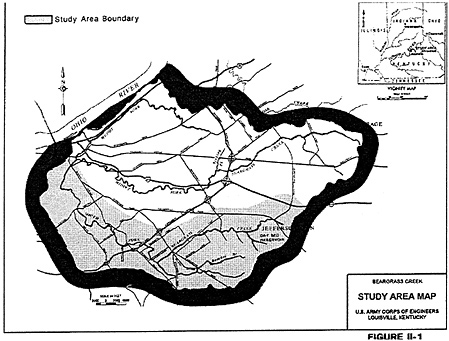
FIGURE 5.1 The Beargrass Creek basin in Louisville, Kentucky. SOURCE: USACE (1997a) (Figure II-1).

about 300 buildings and cause about $7 million in flood damages, while a 100-year flood will impact about 750 buildings and cause about $45 million in flood damages (USACE, 1997c). The expected annual flood damage under existing conditions is approximately $3 million per year.

Flood Damage Reduction Measures

Beargrass Creek has several flood damage reduction structures, the most notable of which is a very large levee at its outlet on the Ohio River ( Figure 5.2a ). This levee was built following a disastrous flood on the Ohio in January 1937, and the levee crest is an elevation of 3 feet above the 1937 flood level on the Ohio River. During the 1937 flood it was reported that “at the Public Library, the flood waters reached a height such that a Statue of Lincoln appeared to be walking on water!” (USACE, 1997b, p. III-2). Near the mouth of Beargrass Creek, a set of

gates can be closed to prevent water from the Ohio River from flowing back up into Louisville. In the event of such a flood, a massive pump station with a capacity of 7,800 cubic feet per second (cfs) is activated to discharge the flow of Beargrass Creek over the levee and into the Ohio River.

Between 1906 and 1943, a traditional channel improvement project was constructed on the lower reaches of the South Fork of Beargrass Creek. It consists of a concrete lined rectangular channel with vertical sides, with a small low-flow channel down the center ( Figure 5.2b ). The channel's flood conveyance capacity is perhaps twice that of the natural channel it replaced, but the concrete channel is a distinctive type of landscape feature that environmental concerns will no longer permit. Other structures have been added since then, including a dry bed reservoir completed in 1980, which functions as an in-stream detention basin during floods.

The proposed flood damage reduction measures for Beargrass Creek form an interesting contrast to traditional approaches. The emphasis of the proposed measures is on altering the natural channel as little as possible and detaining the floodwaters with detention basins. These basins are either located on the creek itself or more often in flood pool areas adjacent to the creek into which excessive waters can drain, be held for a few hours until the main flood has passed, and then gradually return to the creek. Figure 5.2c shows a grassed detention pond area with a concrete weir (in the center of the picture) adjacent to the creek. Figure 5.2d shows Beargrass Creek at this location (a discharge pipe from the pond is visible on the right side of the photograph). Water flows from the creek into the pond over the weir and discharges back into the creek through the pipe. The National Economic Development flood damage reduction alternative on Beargrass Creek called for a total of eight detention basins, one flood wall or levee, and one section of modified channel. Other alternatives such as flood-proofing, flood warning systems, and enlargement of bridge openings were considered but were not included in the final plan.

The evolution of flood damage reduction on Beargrass Creek represents an interesting mixture of the old and the new—massive levees and control structures on the Ohio River, traditional approaches (the concrete-lined channel) in the lower part of the basin, more modern instream and off-channel detention basins in the upstream areas, and local channel modifications and floodwalls. Maintenance and improvement of stormwater drainage facilities in Beargrass Creek are the responsibility of the Jefferson County Metropolitan Sewer District, which is the principal local partner working with the Corps to plan and develop flood damage reduction measures.

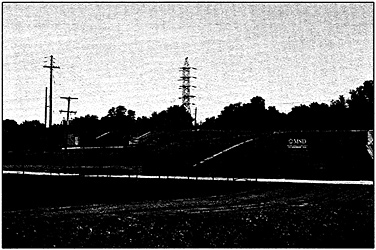
(a) Levee on the Ohio River

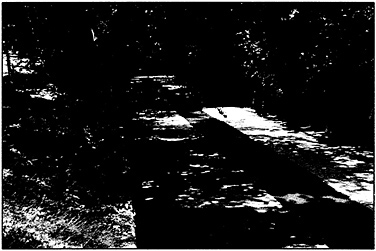
(b) Concrete-lined channel

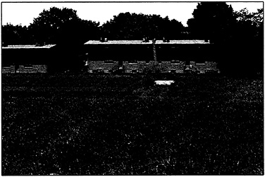
(c) Detention pond

(d) Beargrass Creek at the detention pond

FIGURE 5.2 Images of Beargrass Creek at various locations: (a) the levee on the Ohio River, (b) a concrete-lined channel, (c) a detention pond, and (d) the Beargrass Creek at the detention pond.

In some locations, development has been prohibited in the floodway; but in other places, buildings are located adjacent to the creek. The Corps's feasibility report includes the following comments: “Urbanization continues to alter the character of the watershed as open land is converted to residential, commercial and industrial uses. The quest for open area residential settings in the late 1960s and early 1970s caused a tremendous increase in urbanization of the entire basin. Several developers have utilized the aesthetic beauty of the streambanks as sites for residential as well as commercial developments. This has resulted in increased runoff throughout the drainage area as development has occasionally encroached on the floodplain and, less frequently, the floodway” (USACE, 1997b, p. II-2).

Damage Reaches

To conduct the flood damage assessment, the two main creeks— South Fork of Beargrass Creek and Buechel Branch—are divided into damage reaches. Flood damage and risk assessment results are summarized for each damage reach, and the expected annual damage for the project as a whole is found by summing the expected annual damages for each reach. As shown in Figure 5.3 , the South Fork was divided into 15 damage reaches and the Buechel Branch into 5 reaches (a sixth damage reach on Buechel Branch is not shown in this figure). Approximately 12 miles of Beargrass Creek, and 2.2 miles of Buechel Branch are covered by the these damage reaches. The average length of a damage reach is thus 0.8 miles for the South Fork of the Beargrass Creek, and the average length for Buechel Branch is 0.4 miles. The shorter reaches on Buechel Branch are adjacent to similarly short, upstream reaches in Beargrass Creek where most flood damage occurs. Longer damage reaches are used downstream on Beargrass Creek where less damage occurs.

The highest expected annual flood damage is on Reach SF-9 on the upper portion of the South Fork of Beargrass Creek. Results from this damage reach are used for illustrative purposes at various points in this chapter.

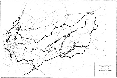
FIGURE 5.3 Damage reaches on the South Fork of Beargrass Creek and Buechel Branch. SOURCE: USACE (1997a) (Figure III-3).

Flood Hydrology

Most of the flood damage reduction measures being considered are detention basins, which diminish flood discharge by temporarily storing floodwater. It follows that the study's flood hydrology component has to be conducted using a time-varying rainfall–runoff model because this allows for the routing of storage water through detention basins. In this case, the HEC-1 rainfall–runoff model from the Corps's Hydrologic Engineering Center (HEC) was used to quantify the flood discharges. The Hydrologic Engineering Center has subsequently released a successor rainfall-runoff model to HEC-1, called HEC-HMS (Hydrologic Modeling System), which can also be used for this type of study (HEC, 1998b).

In each damage reach, and for each alternative plan considered, the risk analysis procedure for flood damage assessment requires a flood – frequency curve defining the annual maximum flood discharge at that location which is equaled or exceeded in any given year with a given probability. In this study all these flood–frequency curves were produced through rainfall–runoff modeling. In other words, a storm of a given

return period was used as input to the HEC-1 model, the water was routed through the basin, and the magnitude of the discharge at the top end of each damage reach was determined (Corps hydrologists have assumed, based on experience in the basin, that storms of given return periods produce floods of the equivalent return period). By repeating this exercise for each of the annual storm frequencies to be considered, a flood–frequency curve was produced for each damage reach. There are eight standard annual exceedance probabilities normally used to define this frequency curve: p = 0.5, 0.2, 0.1, 0.04, 0.02, 0.01, 0.004, and 0.002, corresponding to return periods of 2, 5, 10, 25, 50, 100, 250, and 500 years, respectively. In this study, because even small floods cause damage, a 1-year return period event was included in the analysis and assigned an exceedance probability of 0.999.

Considering that there are 21 damage reaches in the study area and 8 annual frequencies to be considered, each alternative plan considered requires the development of 21 flood–frequency curves involving 168 discharge estimates. During project planning, as dozens of alternative components and plans were considered, the sheer magnitude of the tasks of hydrologic simulation and data assembly becomes apparent.

The hydrologic analysis is further complicated by the fact that the design of detention basins is not simply a cut-and-dried matter. A basin designed to capture a 100-year flood requires a high–capacity outlet structure. Such a basin will have little impact on smaller floods because the outlet structure is so large that smaller events pass through almost unimpeded. If smaller floods are to be captured, a more confined outlet structure is needed, which in turn increases the required storage volume for larger floods. This situation was resolved in the Beargrass Creek study by settling on a 10-year flood as the nominal design event for sizing flood ponds and outlet works. The structures designed in this manner were then subjected to the whole range of floods required for the economic analysis.

Rainfall–Runoff Model

The HEC-1 model was validated by using historical rainfall and runoff data for four floods (March 1964, April 1970, July 1973, February 1990). Modeling results were within 5 percent to 10 percent of observed flows at two U.S. Geological Survey (USGS) streamflow gaging stations: South Fork of Beargrass Creek at Trevallian Way and Middle Fork

of Beargrass Creek at Old Cannons Lane, which have flow records beginning in 1940 and 1944, respectively, and continuing to the present. A total of 42 subbasins were used in the HEC-1 model, and runoff was computed using the U.S. Soil Conservation Service (renamed the Natural Resources Conservation Service in 1994) curve number loss rates and unit hydrographs. The Soil Conservation Service curve numbers were adjusted to allow the matching of observed and modeled flows for the historical events. A 6-hour design storm was used, which is about twice the time of concentration of the basin. The design storm duration chosen is longer than the time of concentration of the basin so that the flood hydrograph has time to rise and reach its peak outflow at the basin outlet while the storm is still continuing. If the design storm is shorter than the time of concentration, rainfall could have ceased in part of the basin before the outflow peaks at the basin outlet. The storm rainfall hydrograph was based on National Weather Service 1961 Technical Paper 40 (NWS, 1961) and on a Soil Conservation Service storm hydrograph, and a 5-minute time interval of computation was used for determining the design discharges.

There is a long flood record of 56 years of data (1940–1996) available in the study area (USGS gage on the South Fork of Beargrass Creek at Trevallian Way). A comparison was made of observed flood frequencies at this site with those simulated by HEC-1, with some adjustment of the older flood data to allow for later development. Traditional flood frequency analysis of observed flow data had little impact in the study. This may have been the case because there was only one gage available within the study area, or because the basin has changed so much over time that the flood record there does not represent homogeneous conditions. Furthermore, the alternatives mostly involve flood storage, which requires computation of the entire flood hydrograph, not just the peak discharge.

Uncertainty in Flood Discharge

Uncertainty in flood hydrology is represented by a range in the estimated flood–frequency curve at each damage reach. In the HEC-FDA program, there are two options for specifying this uncertainty: an analytical method based on the log-Pearson distribution and a more approximate graphical method. The log-Pearson distribution is a mathematical function used for flood–frequency analysis, the parameters of which are determined from the mean, standard deviation, and coefficient

of skewness of the logarithms of the annual maximum discharge data. The graphical method is a flood frequency analysis performed directly on the annual maximum discharge data without fitting them with a mathematical function. In this case the graphical method was used with an equivalent record length of 56 years of data, the length of the flood record of the USGS gage station at Trevallian Way at the time of the study. Figure 5.4 shows the flood–frequency curve for damage reach SF-9 on the South Fork of Beargrass Creek, with corresponding confidence limits based on ± 2 standard deviations about the mean curve.

The confidence limits in this graph are symmetric about the mean when the logarithm to base 10 of the discharge is taken, rather than the discharge itself. This can be expressed mathematically as:

where Q is the discharge value at the confidence limit, log Q is the expected flood discharge, σ log Q is the standard deviation (shown in the rightmost column of Table 5.1 ), and K is the number of standard deviations above or below the mean that the confidence limit lies. Because these confidence limits are defined in the log space, it follows that they are not symmetric in the real flood discharge space. As Table 5.1 shows, the expected discharge for the 100-year flood ( p = 0.01) is 4,310 cfs, the upper confidence limit is 6,176 cfs, and the lower limit is 3,008 cfs. The difference between the mean and the upper confidence limit is thus about 40 percent larger than the difference between the mean and the lower confidence limit. The confidence limits for graphical frequency analysis are computed using a method based on order statistics, as described in USACE (1997d). In this method, a given flood discharge estimate is considered a sample from a binomial distribution, whose parameters p and n are the nonexceedance probability of the flood and the equivalent record length of flood observations in the area, respectively. In this case, n = 56 years, since this is the record length of the Trevallian Way gage.

River Hydraulics

Water surface profiles for all events were determined using the HEC-2 river hydraulics program from the Corps's Hydrologic Engineering Center in Davis, California. Field-surveyed cross sections were obtained

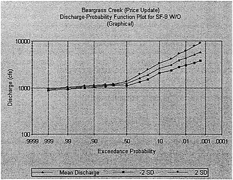
FIGURE 5.4 The flood–frequency curve and its uncertainty at damage reach SF-9 on the South Fork of Beargrass Creek.

at all bridges and at some stream sections near bridges. Maps with a scale of 1 inch = 100 feet with contour intervals of 2 feet were used to define cross sections elsewhere on the stream reaches and were used for measuring the distance between cross sections on the channel and in the left and right overbank areas. Manning's n values for roughness were based on field inspection, on reproduction of known high-water marks from the March 1964 flood on Beargrass Creek, and on reproduction of the rating curve of the USGS gage at Trevallian Way. Manning's equation relates the channel velocity to the channel's shape, slope, and roughness. Manning's n is a numerical value describing the channel roughness. Manning's n values in the concrete channel ranged from 0.015 at the channel invert to 0.027 near the top of the bank. In the natural channels, Manning 's n values ranged from 0.035 to 0.050. In the overbank areas, these values ranged from 0.045 to 0.065. Where buildings blocked the flow, the cross sections were cut off at the effective

TABLE 5.1 Uncertainties in Estimated Discharge Values at Reach SF-9

flow limits. A total of 201 cross sections were used for the South Fork of Beargrass Creek, and 61 cross sections were used for Buechel Branch. The average distance between cross sections was 330 feet on the South Fork of Beargrass Creek and 245 feet on Buechel Branch. Cross sections are spaced more closely than this near bridges and more sparsely in reaches where the cross section is relatively constant.

Figure 5.5 shows the water surface profiles along Beargrass Creek for the eight flood frequencies considered, under existing conditions without any planned control measures. The horizontal axis of this graph is the distance in miles upstream from Beargrass Creek's outlet on the Ohio River. The vertical axis is the elevation of the water surface in feet above mean sea level. The bottom profile in this graph is the channel invert or channel bottom elevation. The top profile is for p = 0.002—the 500-year flood. This particular profile shows a sharp drop near the bottom end of the channel, caused by a bridge at that location that constricts the flow. The flat water surface elevation upstream of the bridge is a backwater effect produced by the inadequate capacity of the bridge opening to convey the flow that comes to it.

For each flood profile computed, the number of structures flooded and the degree to which they are flooded must be assessed. Figure 5.6 shows the locations of the first-floor elevations of structures affected by flooding on the South Fork of Beargrass Creek in relation to several flood water surface profiles under existing conditions. Damage reach SF-9 is located between river miles (RM) 9.960 and 10.363, near the point where there is a sharp drop in the channel bed and water surface elevation on Beargrass Creek. It can be seen that the density of development varies along the channel. Flood damage reduction measures are most effective when they are located close to damage reaches with significant numbers of structures, and they are least effective when they are distant from such reaches.

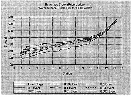
FIGURE 5.5 Water surface profiles for design floods in Beargrass Creek under existing conditions.

Each damage reach has an index location, which is an equivalent point at which all of the damages along the reach are assumed to occur. On reach SF-9, this index location is at river mile 10.124. To assess damages to structures within each reach, an equivalent elevation is found for each structure at the index location such that its depth of flooding at that location is the same as it would have been at the correct location on the flood profile, as shown in Figure 5.7 .

The technique of assigning an elevation at the index location can be far more complex than Figure 5.7 implies, because allowance is made in the HEC-FDA program for the various flood profiles to be nonparallel and also to change in gradient upstream of the index location compared to downstream. In the Beargrass Creek study, a single flood profile for the p = 0.01 event was chosen, and all other profiles were assumed parallel to this one. One damage reach on Beargrass Creek was subdivided into three subreaches to make this assumption more nearly correct. A spatial distribution of buildings over the damage reach is thus converted

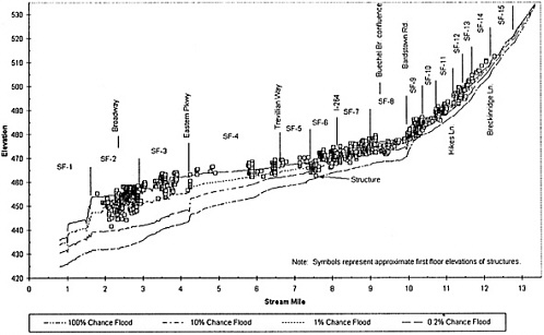
FIGURE 5.6 Locations of structures on floodwater surface profiles along the damage reaches of the South Fork of Beargrass Creek. SOURCE: USACE, 1997c.

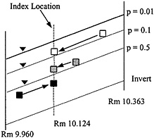
FIGURE 5.7 Assignment of structures to an index location.

into a probability distribution of buildings at the index location, where the uncertainty in flood stage is quantified.

Uncertainty in Flood Stage

The uncertainty in the water surface elevation was quantified by assuming that the standard deviation of the elevation at the index location for the 100-year discharge is 0.5 feet. The 100-year discharge at reach SF-9 is 4,310 cfs, which is the next to last set of points in Fugure 5.8 . To the right of these points, between the 100-year and 500-year flood discharges, the uncertainties are assumed to be constant. For discharges lower than the 100-year return period, the uncertainties in stage height are reduced linearly in proportion to the depth of water in the channel. The various lines shown in Figure 5.8 are drawn as the expected water surface elevation ± 1 or 2 standard deviations determined in this manner.

Economic Analysis

The Corps's analysis of a flood damage reduction project's economic costs and benefits is guided by the Principles and Guidelines ( Box 1.1 provides details on the P&G's application to flood damage reduction

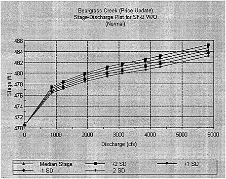
FIGURE 5.8 Uncertainty in the flood stage for existing conditions at reach SF-9 of the South Fork of Beargrass Creek.

studies). According to the P&G , the economic analysis of damages avoided to floodplain structures because of a flood damage reduction project is restricted to existing structures (i.e., federal policy does not allow damages avoided to prospective future structures to be counted as benefits). The P&G do, however, call for the benefits of increased net income generated by floodplain activities after a project has been constructed (so-called “intensification benefits”) to be included in the economic analysis.

Economic analysis of flood damages considers various sorts of flood damage, principal among them being the damage to flooded structures. Information about the structures is quantified using a “structure inventory,” an exhaustive tabulation of every building and other kind of structure subjected to flooding in the study region. A separate computer program called Structure Inventory for Damage Analysis (SID) was used

to evaluate the number of structures flooded as a function of water surface elevation. Structures are divided into four categories: single-family residential, multifamily residential, commercial, and public. A structure is considered to be flooded if the computed flood elevation is above its first-floor elevation. The amount of damage D is a function of the depth of flooding h and the type of structure, and is expressed by a factor, r ( h ), which is equal to a percentage of the value of the structure ( V ) and of its contents (C). This analysis can be expressed as

D = r 1 ( h ) V + r 2 ( h ) C . (5.2)

For residential structures, these damage factors were quantified in 1995 by the Federal Emergency Management Agency (FEMA) using data from flood damage claims. For example, for a one-story house without a basement flooded to a depth of 3 feet, the FEMA estimate is that the damage factors are r 1 = 27% of the value of the structure and r 2 = 35% of the value of the contents. For the same house flooded to a depth of 6 feet, the corresponding damage factors are r 1 = 40% for the structure, and r 2 = 45% for the contents, respectively. The Marshall and Swift Residential Cost Handbook (Marshall and Swift, 1999) was used to estimate the value of single- and multi-family structures (it bears mentioning that the use of standard references such as the Marshall and Swift handbook may potentially represent another source of “knowledge uncertainty ”). The values of their contents were assumed to be 40 percent to 44 percent of the value of the structure. For commercial and public buildings, the values of the structures and their contents were established through personal interviews by Corps personnel. About 85 percent of the structures subject to flood damage are residential buildings.

Types of flood damages beyond those to structures were also considered. For instance, there are several automobile sales lots in the floodplain, and prospective damages to cars parked there during a flood were estimated. Nonphysical damage costs include the costs of emergency services and traffic diversion during flooding. Damage to roads and utilities were also considered.

Uncertainty in Flood Damage

The economic analysis has three sources of uncertainty:

the elevation of the first floor of the building,

the degree of damage given the depth of flooding within the building, and

the economic value of the structure and its contents.

For most structures in Beargrass Creek, the first-floor elevation was estimated from the ground elevation on maps with a scale of 1 inch = 100 feet and with contour intervals of 2 feet. For a sample of 195 structures (16% of the total number), the first-floor elevations were surveyed. It was found that the average difference between estimated and surveyed first-floor elevations of these structures was 0.62 feet.

Corps Engineering Manual (EM) 1110-2-1619 (USACE, 1996b) was used to estimate values for the uncertainties in economic analysis. A standard deviation of 0.2 feet was used to define the uncertainty in first-floor elevations. The uncertainty in the degree of damage given a depth of inundation was estimated by varying the percent damage factor described previously. For residential structures the value of the structure was assigned a standard deviation of 10 percent of the building value, and the ratio of the value of the contents to the structure was allowed to vary with a standard deviation of 20 percent to 25 percent.

For commercial property a separate damage estimate, based on interviews with the owners, was made for each significant property and was expressed as a triangular distribution with a minimum, expected, and maximum damage value for the property. Because every individual structure potentially affected by flooding is inventoried in the damage estimate data, the amount of work required to collect all these damage data was extensive.

The end result of these estimates at each damage reach and damage category is a damage–stage curve (such as Figure 5.9 ) that accumulates the damage to all multifamily structures in this damage reach for various water surface elevations at the index location, denoted by stage on the horizontal axis. This curve is prepared by first dividing the range of the stage (476–486 feet) into increments —increments of 0.5 feet in this case. For each structure, a cycle of 100 Monte Carlo simulations is carried out in which the first-floor elevation and the values of the structure and contents are randomly varied. From these simulations estimates are formed for each 0.5-foot stage height increment of what the expected damage and standard deviation of the damage to that structure would be if the flood stage were to rise to that elevation. For each stage increment, these means and standard deviations are accumulated over all structures in the

reach to form the estimate of the mean and standard deviation of the reach damage ( Figure 5.9 ).

A similar function is prepared for each of the damage categories. At any flood stage, the sum of the damages across all categories is the total flood damage for that reach.

Project Planning

The discussion of the Beargrass Creek study reviewed the technical means by which a particular flood damage reduction plan is evaluated. A plan consists of a set of flood damage reduction measures, such as detention ponds, levees or floodwalls, and channel modifications, implemented at particular locations on the creek. The base plan against which all others are considered is the “without plan,” which means a plan that considers existing conditions in the floodplain and the development expected to occur even in the absence of a flood damage reduction plan. Such development must meet floodplain management policies and have structures elevated out of the 100-year floodplain. A base year of 1996 was chosen for the Beargrass Creek study.

In carrying out project planning, the spatial location of the principal damage reaches is important because flood damage reduction measures located just upstream of or within such reaches have greater economic impact than do flood damage reduction measures located in areas of low flood damage. Project planning also involves a great deal of interaction with local and state agencies, in this case principally the Jefferson County Metropolitan Sewer District.

The Beargrass Creek project planning team consisted primarily of three individuals in the Corps's Louisville district office: a project planner from the planning division, a hydraulic engineer from the hydrology and hydraulics design section, and an economic analyst from the economics branch. The HEC-FDA computer program with risk analysis was carried out by the economic analyst using flood–frequency curves and water surface profiles supplied by the hydrology and hydraulics section and using project alternatives defined by the project planner. The hydrology and hydraulics section was also responsible for the preliminary sizing of potential project structures being considered as plan components. The bulk of the work of implementing the risk analysis aspects of flood damage assessment thus fell within the domain of the Corps economic analyst.

The HEC-FDA program is applied during the feasibility phase of

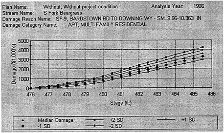
FIGURE 5.9 The damage–stage curve with uncertainty for multifamily residential property in Reach SF-9 of the South Fork of Beargrass Creek.

flood damage reduction planning. This had been preceded by a reconnaissance phase, a preliminary assessment of whether reasonable flood damage reduction planning can be done in the area. As explained in Chapter 2 , the reconnaissance phase is fully funded by the federal government, but the feasibility phase must have half the costs met by a local sponsor. Assuming the feasibility phase yields an acceptable plan and additional funds are authorized, the project proceeds to a detailed design and construction phase, which also requires local cost sharing. The Beargrass Creek project is now (as of May 2000) in the detailed design phase.

Evaluation of Project Alternatives

Expected annual flood damages in Beargrass Creek under existing conditions are estimated to be $3 million. Project benefits are calculated as the difference between this figure and the lower expected annual damages that result with project components in place. Project costs are annualized values of construction costs discounted over a 50-year period using an interest rate of 7.625 percent. Project net benefits are the differ-

ence between project benefits and costs. For components to be included in the project, they must have positive net benefits.

The first step in evaluating project alternatives is to consider each component flood damage reduction measure by itself to see if it yields positive net benefits. A total of 22 components were examined individually, 11 on the South Fork of Beargrass Creek and 11 on Buechel Branch. All 11 of the South Fork components were economically justified on a stand-alone basis. Only 3 of the 11 components on Buechel Branch were justified individually: the other 8 components were thus deleted from further consideration.

The next step is to formulate the National Economic Development (NED) plan. In theory, this is supposed to proceed by selecting first the component with the largest net benefits, adding the component with the next largest net benefits, evaluating them together, and continuing to add more components until the combined set of components has the largest overall net benefits. It turned out that this idealized approach could not be used at the South Fork of Beargrass Creek because of economic and hydraulic interactions among the components. The study team commented: “Therefore, the formulation process was different and more complicated than originally anticipated. The study team could not follow the incremental analysis procedure to build up the NED plan because the process became a loop of H&H computer runs. Our component with the greatest net benefits is located near the midpoint of the stream; thus, each time we would add a component upstream it would affect all components downstream and vice versa. We could never truly optimize or identify the plan which produces the greatest net benefits” (USACE, 1997c, p. IV-62).

The problems were further complicated by the fact that there are three separate sections of the study region: the South Fork of Beargrass Creek and Buechel Branch upstream of their junction and the South Fork downstream of this junction ( Figure 5.3 ). In the downstream region, flood damage reduction measures on the upper South Fork and Buechel Branch compete for project benefits by reducing flood damages. The result of these complications is that the plan was built up incrementally by separately considering the three sections of the region. First, the most upstream control structure in each section was selected, then structures downstream were added. At the end—when the components from the three sections had been aggregated into a single overall plan—it was determined whether the plan could be improved by omitting individual marginal components. The end result of this iterative process was a recommended plan with 10 components: 8 detention basins, 1 floodwall,

and 1 channel improvement.

Each plan has to be evaluated using the Monte Carlo simulation process. The number of simulations varies by reach, with 10,000 required for Reach SF-9 and with a range of 10,000–100,000 required for the other reaches. On a 300 MHz Pentium computer, evaluation of a single plan takes about 25 minutes of computation time.

Risk of Flooding

The HEC-FDA program also produces a set of statistics that quantify the risk of being flooded in any reach for a given plan, as shown in Table 5.2 . For reach SF-9, the target elevation is 477.2 feet, which is the elevation of the overbank area in this reach. The probability estimates shown are annual exceedance probability and conditional nonexceedance probability. The annual exceedance probability refers to the risk that flooding will occur considering all possible floods in any year. The conditional nonexceedance probability describes the likelihood that flooding will not occur during a flood of defined severity, such as the 100-year (1 percent chance) flood.

There is a subtle but important distinction between these two types of risk measures. The annual exceedance probability accumulates all the uncertainties into a single estimate both from the natural variability of the unknown severity of floods and from the knowledge uncertainty in estimating methods and computational parameters. The conditional non-exceedance probability estimate divides these two uncertainties, because it is conditional on the severity of the natural event and thus represents only the knowledge uncertainty component. In this sense, the conditional nonexceedance probability corresponds most closely to the traditional idea of adding 1 foot or 3 feet on the 100-year base flood elevation, while the annual exceedance probability corresponds more closely to the goal of ensuring that the chance of being flooded is less than a given value, such as 1 percent, considering all sources of uncertainty.

The “target stage annual exceedance probability” values in Table 5.2 are the median and the expected value or mean of the chance that flooding will occur in any given year for the various reaches. Thus, for reach SF-9, there is approximately a 36 percent chance that flooding will occur beyond the target stage in any given year, while in reach SF-14 upstream, that chance is only about 9 percent. The “long term risk” values in the

TABLE 5.2 Risk of Flooding in Damage Reaches Calculated Uncertainty for 1996 at Beargrass Creek

figure refer to the chance (Rn) that there will be flooding above the target stage at least once in n years, determined by the formula

R n = 1− (1− p e ) n , (5.3)

where p e is the expected annual exceedance probability. For example, for reach SF-9, where p e = 0.3640, for n = 10 years, R 10 = 1− (1 − 0.3640) 10 = 0.9892, as shown in Table 5.2 .

The conditional nonexceedance probability values shown on the right-hand side of Table 5.2 are conditional risk values that correspond to the reliability that particular floods can be conveyed without causing damage in this reach. Thus, in reach SF-9, a 10 percent chance event (10-year flood) has about a 0.27 percent chance of being conveyed without exceeding the target stage, while for a 1 percent chance event (100-year flood), there is essentially no chance that it will pass without exceeding the target stage. By contrast, in Reach SF-14 at the upstream end of the study area, the conditional nonexceedance probability of the reach passing the 10-year flood is about 52 percent; that of the reach passing the 100-year flood is about 100 percent. As the flood severity increases, the chance of a reach being passed without flooding diminishes.

Effect on Project Economics of Including Risk and Uncertainty

The HEC-FDA program that includes risk and uncertainty factors in project analysis became available to the Beargrass creek project team late in the study period. Before then, the team used an earlier economic analysis program (Expected Annual Damage, or EAD) which computed expected annual damages without these uncertainties. O' Leary (1997) presented the data shown in Table 5.3 to compare the two approaches. It is evident that including risk and uncertainty increases the expected annual damage both with and without flood damage reduction plans. The net effect of their inclusion on the Beargrass Creek project is to increase the annual flood damage reduction benefits from $2.078 million to $2.314 million. The study team made a comparison between the components included in the National Economic Development plan in the two computer programs and found that there was no change. Hence, although the inclusion of risk and uncertainty increased project benefits, it did not result in changing the flood damage reduction components included in the National Economic Development plan.

O'Leary (1997) also presented statistics of the project benefits derived from the HEC-FDA program for the National Economic Development plan. The expected annual benefits of the National Economic Development plan—$2.314 million—are the same in Table 5.3 and Table 5.4 . The net benefits in the fourth column of Table 5.4 are found by subtracting the annual project costs from the expected annual benefits; the benefit-to-cost ratio is the ratio of the expected benefits to costs.

The 25 th percentile, median (50 th percentile), and 75 th percentile of the expected annual benefits are also shown. The project net benefits are positive at all levels of assessment, and all benefit-to-cost ratios are greater than 1.00. It is interesting to see that the median expected annual benefits ($2.071 million) are nearly the same as the expected value of these benefits without considering uncertainty ($2.078 million). Moreover, the expected value ($2.314 million) is greater than the median, and the difference between the 75 th percentile and the median is greater than the difference between the median and the 25 th percentile. All these characteristics point to the fact that the distributions of flood damages and of expected annual benefits are positively skewed when uncertainties in project hydrology, hydraulics, and economics are considered. This is why the project benefits increase when these uncertainties are considered. The project benefits for the 25 th percentile, 50 th percentile, and 75 th percentile in Table 5.4 should be read with caution because they are compiled for the project by adding together the corresponding values for all the damage reaches. The percentile value of a sum of random variables is not necessarily equal to the sum of the percentile values of each variable.

TABLE 5.3 Expected Annual Damages (EAD) With and Without Uncertainty in Damage Computations (millions of dollars per year)

TABLE 5.4 Statistics of project benefits under the NED plan using the HEC-FDA Program

RED RIVER OF THE NORTH AT EAST GRAND FORKS, MINNESOTA, AND GRAND FORKS, NORTH DAKOTA

A devastating flood occurred at East Grand Forks, Minnesota, and Grand Forks, North Dakota, in April 1997. After the flood, flood damage reduction studies previously done for the two cities were combined into a joint study, and risk analysis was performed to evaluate the reliability of the proposed alternatives and to evaluate their economic impacts. A risk analysis study performed before the flood was presented in a paper at the Corps's 1997 Pacific Grove, California, workshop (Lesher and Foley, 1997). This paper and subsequent analysis (USACE, 1998a, b, c), as well as a visit to the Corps's St. Paul district office by a member of this committee, form the basis of this discussion of the East Grand Forks–Grand Forks study.

East Grand Forks, Minnesota, and Grand Forks, North Dakota, are located on opposite banks of the Red River of the North and are approximately 300 miles above the river's mouth at Lake Winnipeg, Manitoba, Canada ( Figure 5.10 ). The East Grand Forks–Grand Forks metropolitan area has a population of approximately 60,000 and is located about 100 miles south of the U.S.–Canadian border. The total drainage area of the East Grand Forks–Grand Forks basin is 30,100 square miles. Included in this drainage area is the Red Lake River subbasin that effectively drains about 3,700 square miles in Minnesota and joins the mainstream of the Red River at East Grand Forks. The study area of East Grand Forks–Grand Forks lies in the middle of the Red

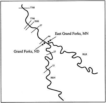
FIGURE 5.10 Schematic of the Red River of the North (RRN) and Red Lake River (RLR) at the East Grand Forks, Minnesota and Grand Forks, North Dakota study area. Numbers indicate USGS stream gages.

River Valley. The valley is exceptionally flat with a gradient that slopes 3–10 feet per mile toward the river with the north–south axis having a gradient of about three-quarters of a foot per mile. The valley extends approximately 23 miles west and 35 miles east of East Grand Forks– Grand Forks and is a former glacial lake bed.

Both cities have a long history of significant flooding from the Red River of the North and the Red Lake River. The most damaging flood of record occurred in April 1997 (see Table 5.5 ), when the temporary levee systems and flood-fighting efforts of both communities could not hold back the floodwaters of the Red River. The resulting damages were disastrous and affected both cities dramatically. Total damages to existing structures and contents during the 1997 flood were estimated to exceed $800 million. An additional $240 million was spent for emergency-related costs.

TABLE 5.5 Maximum Recorded Instantaneous Peak Flows; Red River of the North at Grant Forks, North Dakota

Risk Analysis

A risk analysis for the proposed flood damage reduction project for the Red River of the North at East Grand Forks, Minnesota, and Grand Forks, North Dakota, used a Latin Hypercube analysis to sample interactions among uncertain relationships associated with flood discharge and elevation estimation. Latin Hypercube is a stratified sampling technique used in simulation modeling. Stratified sampling techniques, as opposed to Monte Carlo-type techniques, tend to force convergence of a sampled distribution in fewer samples. Because the Hydrologic Engineering Center Flood Damage Analysis program (HEC-FDA) was new at the time, and in the interest of saving time, the analysis was performed using a spreadsheet template. The flood damage reduction alternatives analyzed included levees of various heights and a diversion channel in conjunction with levees. The project reliability option in the HEC risk spreadsheet was used to determine the reliability of the alternative levee heights and of the diversion channel in conjunction with levees. The following sections discuss the sensitivity in quantifying the uncertainties and the representation of risk for the alternatives.

Discharge–Frequency Relationships

The log-Pearson Type III distribution, recommended in the Water Resource Council's Bulletin 17B (IACWD, 1981) and incorporated

within the Corps's HEC Flood Frequency Analysis (HEC-FFA) computer program, was used for frequency analysis of maximum annual streamflows, and the noncentral t distribution was used for the development of confidence limits. Discharge–frequency relationships were needed for both the levees and the diversion channel in combination with levees. An analysis (coincidental frequency) was performed to develop the discharge– frequency curves for the Red River of the North downstream and upstream of the Red Lake River for the levees only condition. A graphical method was used to develop the discharge–frequency curves for the diversion channel in combination with levees. Details of these procedures can be found in a Corps instruction manual from the St. Paul district (USACE, 1998a). A brief discussion of these procedures is provided below.

The Grand Forks USGS stream gage (XS 44) is currently located 0.4 miles downstream from the Red Lake River in Grand Forks, North Dakota ( Figure 5.10 ). The discharge–frequency curve for this station along with the 95 percent and 5 percent confidence limits (90% confidence band) are plotted in Figure 5.11 . An illustration of the noncentral t probability density function for the 1 percent event is also shown in that figure. Selected quantities of that discharge–frequency relationship are shown in column 2 of Table 5.6 . The coincidental discharge–frequency relationship for the Red River just upstream of the mouth of the Red Lake River (column 3 of Table 5.6 ) was computed with the HEC-FFA computer program. The basic flow values were obtained by routing the 96 years of available data on Red Lake River flows from Crookston (55 miles upstream of the mouth) downstream to Grand Forks. The resulting flows were subtracted from the Red River at Grand Forks flows to obtain coincident discharges on the Red River upstream of Red Lake River. The two-station comparison method of Bulletin 17B was used to adjust the logarithmic mean and standard deviation of this short record (96 years) based on regression analysis with the long-term record at the Grand Forks station (172 years). Correlation of coincident flows for the short record with concurrent peak flows for the long record produced a correlation coefficient of 0.975.

Adjustment of the statistics yielded an equivalent record length of 165 years. The adopted coincidental discharge–frequency curve for the Red River upstream of the Red Lake River is shown in column 3 of Table 5.6 for selected annual exceedance probabilities. The coincidental discharge –frequency curve for the Red Lake River at the mouth was determined by computing the difference in Red River flows both upstream and downstream of Red Lake River (see column 4 in Table 5.6 ). Statistics for the adopted relationship were approximated by synthetic methods presented in Bulletin 17B (for more details, see USACE (1998a)).

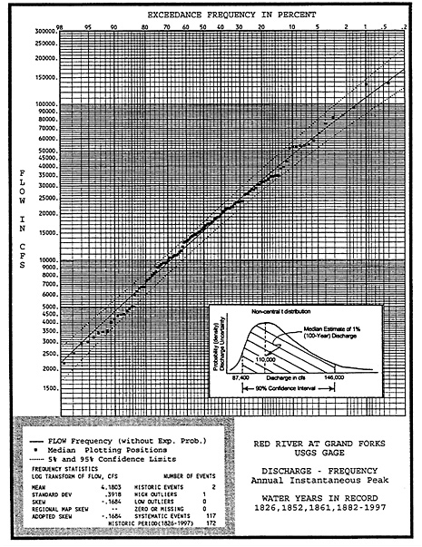
FIGURE 5.11 Flood (discharge) frequency curve for the Red River at Grand Forks.

TABLE 5.6 Instantaneous Annual Peak Discharges (cfs) and their Annual Exceedance Probabilities (%) — Existing Conditions

and downstream of Red Lake River (see column 4 in Table 5.6). Statistics for the adopted relationship were approximated by synthetic methods presented in Bulletin 17B (for more details, see USACE (1998a)).

The Plan Comparison Letter Report developed in February 1998 for flood damage reduction studies for East Grand Forks, Minnesota, and Grand Forks, North Dakota, evaluated an alternative flood damage reduction plan that included a split-flow diversion channel along with permanent levees. The discharge–frequency relationships for the modified conditions, shown in Table 5.7 , were developed as follows. The modified-condition discharge–frequency curve for the Red River upstream of Red Lake River was graphically developed based upon the operation of the diversion channel inlet. Red River flows are not diverted until floods start to exceed those having return periods of 5 years (20% annual exceedance probability). The channel is designed to continue to divert Red River flows at a rate that allows the design flood (0.47%) discharge of 102,000 cfs (upstream of the diversion) to be split such that 50,500 cfs is diverted and 51,500 cfs is passed through the cities. This operation is reflected in the modified discharge–frequency relationship shown in Table 5.7 for the Red River upstream of Red Lake River (columns 2 and

TABLE 5.7 Instantaneous Annual Peak Discharges (cfs) and their Annual Exceedance Probabilities (%)—Condition with Diversion Channels

3).Synthetic statistics (mean, standard deviation, and skewness) in accordance with methodology presented in Bulletin 17B were computed for the discharge-frequency relationships of the below-diversion flows.

The modified-condition discharge–frequency curve for the Red River downstream of Red Lake River was graphically computed based upon the operation of the diversion channel. The modified-condition Red River discharges upstream of Red River were added to the coincident flows on Red Lake River (column 4). The resulting discharges were plotted for graphical development of the modified-condition discharge– frequency relationship for the Red River downstream of Red Lake River and are summarized in Table 5.7 (column 5). Synthetic statistics for this discharge–frequency relationship were computed for use in the risk analysis.

Elevation–Discharge Relationships

The water surface elevations computed using the HEC-2 computer program are shown in Table 5.8 for three cross sections (7790, 7800, and 7922) corresponding to the previous USGS gage locations and for cross

section 44, which corresponds to the current USGS gage location (see Figure 5.10 for the cross section locations). These computed water surface elevations (CWSE) were based on the expected discharge quantities from the coincidental frequency analysis performed in June 1994 for the Grand Forks Feasibility Study. These data were used to transfer observed elevations from previous USGS gage sites to the current site (cross section 44) at river mile 297.65, and they were used in determining the elevation –discharge uncertainty. The water surface profile analysis was performed using cross-sectional data obtained from field surveys. Data were also obtained from field surveys and from USGS topographic maps. The HEC-2 model was calibrated to the USGS stream gage data and to high-water marks for the 1969, 1975, 1978, 1979 and 1989 flood events throughout the study area. Note that these water surface elevations assume the existing East Grand Forks and Grand Forks emergency levees are effective. The levees were assumed effective because through extraordinary efforts, they have generally been effective for past floods with the exception of the 1997 flood.

Ratings at stream gage locations provide an opportunity to directly analyze elevation–discharge uncertainty. The measured data are used to derive the “best fit” elevation-discharge rating at the stream gage location, which generally represents the most reliable information available. In this study, the adopted rating curve for computing elevation uncertainty is based on the computed water surface elevations from the calibrated HEC-2 model shown in Table 5.8 .

This adopted rating curve for cross section 44 at the current USGS gage is shown in Figure 5.12 . Measurements at the gage location were used directly to assess the uncertainty of the elevation–discharge relationship. The normal distribution was used to describe the distribution of error from the “best-fit” elevation–discharge rating curve. The observed gage data (for the four cross sections presented in Table 5.8 ) were transferred to the current gage site at river mile 297.65 based on the gage location adjustments presented in Table 5.9 , which were computed from the water surface elevations in Table 5.8 . These adjustments were plotted against the corresponding discharge below the Red Lake River, and curves were developed to obtain adjustments for other discharges.

The deviations of the observed elevations from the fitted curve were used to estimate the uncertainty of the elevation–discharge rating curve shown in Figure 5.11 . The deviations reflect the uncertainty in data values as a result of changes in flow regime, bed form, roughness/resistance to flow, and other factors inherent to flow in natural streams. Errors also

TABLE 5.8 Computed Water Surface Elevations of the Red River of the North at Grand Forks, North Dakota (units in feet above sea level)

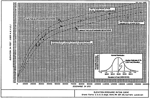
FIGURE 5.12 Rating curve (water elevation vs. discharge)for the Red River at Grand Forks.

TABLE 5.9 Adjustments Used in Transferring Observed Elevations from Previous USGS Gage Sites to Current Gage Site at RM 297.65 (XS 44)

result from field measurements or malfunctioning equipment. A minimum of 8–10 measurements is normally required for meaningful results. The measure used to define the elevation–discharge relationship uncertainty is the standard deviation:

Where X = observed elevation adjusted to current gage location (if 5.12 necessary), M = computed elevation from adopted rating curve, and N = number of measured discharge values (events).

The elevation uncertainty was computed for two different discharge ranges for this analysis. Based on the observed elevations plotted on the adopted rating curve, it appeared that there was greater uncertainty for discharges less than about 10% of annual exceedance probability event due to ice effects on flow. Therefore, the standard deviation was computed for discharges greater than between 22,000 cfs, which corresponds approximately to the zero damage elevation based on the adopted rating curve, and 44,000 cfs, which is slightly greater than the 10 percent annual exceedance probability. The standard deviation was also computed for discharges greater than 50,000 cfs. During the period of record, there were 25 events with a discharge between 22,000 and 44,000 cfs and 10 events with a discharge greater than 50,000 cfs. The standard deviation was 1.66 feet for discharges between 22,000 and 44,000 cfs and was 1.55

feet for discharges greater than 50,000 cfs. In the risk and uncertainty simulations, the standard deviation was linearly interpolated between 1.66 and 1.55 feet for discharges between 44,000 and 50,000 cfs. (See USACE (1998b) for more details.)

In an earlier risk analysis that was performed for the Grand Forks Feasibility Study, a much lower standard deviation of 0.50 feet was used for discharges greater than 50,000 cfs. However, adding the 1997 flood to the analysis resulted in a standard deviation of 1.55 feet, which is similar to that computed for discharges less than 44,000 cfs. It should be noted that the discharge and elevation used in this analysis for the 1997 flood was the peak discharge of 136,900 cfs occurring on April 18, 1997 (see Table 5.4 ), and an elevation of 831.21 feet (Stage 52.21). The peak elevation of 833.35 feet (Stage 54.35) occurred on April 22, 1997 at a discharge of 114,000 cfs. The elevation of 831.21 feet was almost 5 feet below the rating curve at a discharge of 136,900 cfs; however, the peak elevation of 833.35 feet at a discharge of 114,000 cfs was essentially on the adopted rating curve. Both of these points are plotted on the rating curve in Figure 5.12 . Lines representing ± 2 standard deviations for the normal distribution, which encompasses approximately 95 percent of all possible outcomes, are also shown on the rating curve. An illustration of the normal distribution at the 1 percent (100-year) event for the project levee condition is also shown in Figure 5.12 .

Risk and Uncertainty Analysis Results

Four index locations were selected to evaluate project performance and project sizing. These locations are cross sections 57, 44 (current USGS gage), 27, and 15 ( Figure 5.10 ). The four locations were selected based on economic requirements for project sizing (see USACE, 1998c). The elevation–discharge rating curves (based on HEC-2 analysis) for existing and project conditions at these locations can be found in the USACE (1998b). Each of these rating curves shows three conditions, where applicable: (1) existing conditions, (2) removal of the pedestrian bridge at cross sections 7920-7922 and with project levees (“levee only”); and (3) with removal of the pedestrian bridge, with project levees, and with the diversion channel (“diversion channel”). Existing conditions means that the existing emergency levees are assumed to be effective up to and including the 5 percent (20-year) event and are ineffective for larger floods. The 5 percent (20-year) event was selected based

on comparison of water surface profiles with effective and probable failure point (PFP) levee elevations provided by the Geotechnical Design Section analysis (see USACE, 1998b, paragraph A.2.11 and Appendix B of this report). The pedestrian bridge was removed based on input from the cities of East Grand Forks and Grand Forks. The rating curves for the diversion channel alternative were based on limited information. The Red River to the North would start to divert into the diversion channel at the 20 percent (5-year) flood; therefore, up to this point the rating curve for existing conditions with levees was used.

An additional location was also selected to evaluate the performance of the levee only and diversion channel with 1 percent (100-year) levee alternatives. This location is at cross section 7700 at the downstream end of the project levees (see Figure 5.10 ). Cross section 7700 was selected based on hydraulic analysis as the least critical location—the location where the levees in combination with the diversion channel would first overtop from downstream backwater (see USACE, 1998b).

Project Reliability

The project reliability results are summarized in Table 5.10 , Table 5.11 through Table 5.12 . Table 5.9 contains the results for the levees-only alternatives. Table 5.11 contains the results for the diversion channel in combination with 1 percent (100-year) levees. Note that in Table 5.10 , three different alternative top-of-levee heights are evaluated, whereas in Table 5.11 , it is always the same alternative—diversion channel with 1 percent levees— but for the three different events. The top-of-levee elevations were computed based on a water surface elevation profile to ensure initial overtopping would occur at the least-critical location (here, cross section 7700). The downstream top-of-levee elevations were selected with the intent of having 90 percent probability of containing the specified flood and were based on previous risk analysis for the Grand Forks Feasibility Study preliminarily updated to include the 1997 flood. The 2 percent (50-year), 1 percent (100-year), and 0.47 percent (210-year/1997 flood) top-of-levee profiles are 3.2, 3.4, and 2.7 feet above their respective water surface profiles at the downstream end ( Table 5.10 ).

As seen in Table 5.10 , the intent of having 90 percent probability of containing the specified flood is generally realized. The 2 percent levees have a 92 percent probability of containing the 2 percent flood. The 1 percent levees have a 90 percent probability of containing the 1 percent

flood. The 0.47 percent levees have an 87 percent probability of containing the 0.47 percent flood.

TABLE 5.10 Reliability at Top of Levee for Three Top-of-Levee Heights

TABLE 5.11 Project Reliability at Top of Levee for Diversion Channel with 1 Percent (100-Year) Levees for Three Different Events

Reliability results for the diversion channel with 1 percent levees are summarized in Table 5.11 . Note again that the levees constructed in combination with the diversion are the same as for the 1 percent flood without the diversion channel and are the same for all three floods analyzed. As seen in the table, there is a 99 percent or greater probability of containing the flood for all three floods considered when the project includes the diversion channel.

As previously noted, the most critical location for project performance is at cross section 7700 at the downstream end of the project. Table 5.12

summarizes the results for all the alternatives considered and for numerous floods. The probability of the diversion channel in combination with 1 percent levees for the 0.2 percent event is listed in the table as greater than 95%. A more specific reliability was not cited for the 0.2 percent event for two reasons: (1) the discharge–frequency curve based on the approximate statistics starts to diverge from the graphical curve for extreme events and, (2) there was limited information available to develop the Red River to the North rating curves for the diversion alternative. These reasons are also why more extreme events were not analyzed.

TABLE 5.12 Conditional Exceedance Probability of Alternative for Various Events (based on analysis at downstream end of project—XS 7700)

Table 5.13 presents the simulated conditional exceedance probabilities from the economic project sizing analysis. The without-project condition is also included in this table for comparison purposes. The without-project condition is based on a zero damage elevation of 824.5 feet, assumes credit is given to the existing levees, and assumes all properties that were substantially damaged (50% or more damage) in the 1997 flood have been removed.

Based on the above analysis of alternative plans and further economic and environmental considerations, the recommended National

TABLE 5.13 Residual Risk Comparison

Economic Development (NED) plan consists of a permanent levee and floodwall system designed to reliably contain the 210-year flood event. This equates to an 87.7 percent reliability of containing the 210-year flood event ( Table 5.12 ) and would reliably protect against a flood of the magnitude of the 1997 flood.

The recommended plan would remove protected areas from the regulatory floodplain, increase recreational opportunities, and enhance the biological diversity in the open space created. The recommended plan anticipates the need to acquire over 250 single-family residential structures, 95 apartment or condominium units, and 16 businesses along the current levee/floodwall alignment.

The total cost of the recommended multipurpose project is $350 million including recreation features and cultural resources mitigation costs. The federal share of the project would be $176 million and the nonfederal share would be $174 million. The benefit-to-cost ratio has been calculated as 1.07 for the basic flood reduction features of the project and as 1.90 for the separable recreation features (USACE, 1998b). The recommended project has an overall benefit-to-cost ratio of 1.10.

The cities of East Grand Forks, Minnesota, and Grand Forks, North Dakota, will serve as the project's nonfederal sponsors. Through legislation, the State of Minnesota has committed to provide financial support in the form of bonds and returned sales taxes to the city of East Grand Forks. In verbal and written comments from its governor, the State of North Dakota has committed to provide financial assistance to the city of Grand Forks.

Reducing flood damage is a complex task that requires multidisciplinary understanding of the earth sciences and civil engineering. In addressing this task the U.S. Army Corps of Engineers employs its expertise in hydrology, hydraulics, and geotechnical and structural engineering. Dams, levees, and other river-training works must be sized to local conditions; geotechnical theories and applications help ensure that structures will safely withstand potential hydraulic and seismic forces; and economic considerations must be balanced to ensure that reductions in flood damages are proportionate with project costs and associated impacts on social, economic, and environmental values.

A new National Research Council report, Risk Analysis and Uncertainty in Flood Damage Reduction Studies , reviews the Corps of Engineers' risk-based techniques in its flood damage reduction studies and makes recommendations for improving these techniques. Areas in which the Corps has made good progress are noted, and several steps that could improve the Corps' risk-based techniques in engineering and economics applications for flood damage reduction are identified. The report also includes recommendations for improving the federal levee certification program, for broadening the scope of flood damage reduction planning, and for improving communication of risk-based concepts.

Welcome to OpenBook!

You're looking at OpenBook, NAP.edu's online reading room since 1999. Based on feedback from you, our users, we've made some improvements that make it easier than ever to read thousands of publications on our website.

Do you want to take a quick tour of the OpenBook's features?

Show this book's table of contents , where you can jump to any chapter by name.

...or use these buttons to go back to the previous chapter or skip to the next one.

Jump up to the previous page or down to the next one. Also, you can type in a page number and press Enter to go directly to that page in the book.

Switch between the Original Pages , where you can read the report as it appeared in print, and Text Pages for the web version, where you can highlight and search the text.

To search the entire text of this book, type in your search term here and press Enter .

Share a link to this book page on your preferred social network or via email.

View our suggested citation for this chapter.

Ready to take your reading offline? Click here to buy this book in print or download it as a free PDF, if available.

Get Email Updates

Do you enjoy reading reports from the Academies online for free ? Sign up for email notifications and we'll let you know about new publications in your areas of interest when they're released.

Future Strategies

State Case Studies

Federal Review

Management Goals

• Holistic Approach to Coastal FRM

CONTENTS ≡

CONTENTS ✕

Coastal Management Program

Shoreline regulations, floodplain management, wetland management, building codes, community planning, stormwater and runoff management, erosion management, climate adaptation initiatives, state management capacity, alternatives to structural mitigation, long-term planning, balance of mitigation and disaster recovery, holistic management approach, new york coastal flood risk management case study.

Policies and Programs

The New York Coastal Management Program , established in 1982, is housed within the New York Department of State’s Office of Planning, Development, and Community Infrastructure . Much of the program’s legislative authority is drawn from the state Waterfront Revitalization of Coastal Areas and Inland Waterways law as well as the Coastal Erosion Hazard Areas law . The program pursues goals related to coastal resources protection and development, local waterfront revitalization, coordination of major activities affecting coastal resources, public awareness of coastal issues, and federal consistency with state coastal management policies. Within New York, the Department of State administers the program and coordinates its implementation in cooperation with the state Department of Environmental Conservation as well as other state agencies.

Coastal program boundaries extend along the coast of Long Island, New York City, Hudson River estuary, both Great Lakes that border New York, and the Niagara River. Specific landward boundaries of the coastal program vary by region and locality due to initial delineation proposals from local government agencies. All barrier and coastal islands on Long Island are included within program boundaries along with areas 1,000 feet landward of the shoreline, extending further in some cases. The New York City program boundary generally extends 500 to 1,000 feet inland from the shoreline, with select areas along major tributaries also extending further. Within the Hudson River Valley the landward boundary is generally 1,000 feet but may extend up to 10,000 feet in areas that possess high aesthetic, agricultural, or recreational value. In the Great Lakes region the boundary is also generally 1,000 feet, though urbanized areas or transportation infrastructure parallel to shore limit the boundary to 500 feet or less in some cases.

Coastal management program consistency reviews require federal actions in the state coastal zone to be consistent with the enforceable policies of the state program or the policies of an approved local waterfront revitalization program. The program also contains provisions to ensure consistency of state actions in coastal areas. Of the 44 coastal management program enforceable policies in New York, seven specifically address flooding and erosion hazards. These policies touch on a number of aspects of coastal flood risk management including the siting of buildings in coastal areas to minimize risk to property and human lives, protection of natural features that mitigate coastal flood risk, construction of erosion control structures to to meet long-term needs, prevention of flood level increases due to coastal activities or development, prevention of coastal mining or dredging from interfering with natural coastal processes, use of public funds for erosion protection structures, and use of non-structural mitigation measures when possible. Additional enforceable policies address coastal development, fish and wildlife resources, public access, recreation, historic and scenic resources, agricultural lands, energy and ice management, water and air resources, and wetlands management.

At the state level, aspects of New York’s Environmental Conservation Law , Local Waterfront Revitalization Program , and State Environmental Quality Review permitting program influence coastal zoning and development decisions. Article 34 of the Environmental Conservation Law requires the identification of coastal erosion hazard areas and rates of recession of coastal lands. Shoreline setbacks must then be implemented at a distance that is sufficient to minimize damage from erosion. Article 36 of the Environmental Conservation Law , the state Flood Plain Management Act, also addresses coastal hazards, requiring walled and roofed buildings to be sited landward of mean high tide and prohibiting mobile homes within coastal high hazard areas, among other restrictions. Article 15, Water Resources Law , regulates the placement of coastal structures such as docks or piers and also addresses the placement of fill in coastal areas. Together these elements of the Environmental Conservation Law provide much of the legal basis for zoning decisions that can affect coastal flood risk at the municipal and local level.

Participation in the Local Waterfront Revitalization Program can also influence a local government’s coastal zoning decisions. In the process of preparing and adopting a revitalization program, local governments provide a more specific implementation of the state Coastal Management Program, taking advantage of local regulatory powers such as zoning ordinances and site plan review. Upon approval of a Local Waterfront Revitalization Program, state actions must then be consistent with the local program. In this way the enforceable policies of the Coastal Management Program, including those that relate to coastal flooding and erosion, are incorporated into local zoning decisions. Elements of enforceable policies are also incorporated into environmental permitting through the State Environmental Quality Review Program, which requires state agencies and local governments to prepare an environmental impact statement for any action that may have a significant impact on the environment. If an action in a coastal area requires the preparation of an impact statement, it must also be determined that the action is consistent with any relevant coastal enforceable policies. Consistency reviews must also be applied to NYS SEQRA type 1 actions as well as unlisted actions.

Floodplain management activities within New York are primarily conducted through the National Flood Insurance Program . Any regulations developed by the state must be at a minimum as strict as those prescribed by FEMA. Beyond the state level communities may adopt more restrictive floodplain management regulations. Within the state, local communities largely regulate development within federally designated Special Flood Hazard Areas, with state assistance provided by the New York State Department of Environmental Conservation. Local development permits govern private development within floodplains as well as development by a county, city, town, village, school district, or public improvement district, as specified in the state Environmental Conservation Law.

State standards for floodplain development permits in all designated special flood hazard areas require adequate anchorage and use of flood resistant material for all new construction and substantial improvement to existing structures. Utilities must also be designed in a manner that minimizes or eliminates risk of damage or failure during flood events. In areas where base flood elevation data exists, new construction or substantially improved residential structures must have the lowest floor at two feet above the BFE, including basements and cellars. Nonresidential structures may employ floodproofing to provide protection. Any enclosed areas below the base flood elevation must be designed to allow for the equalization of hydrostatic forces on exterior walls during a flood event. If no base flood elevation has been determined, new construction or substantially improved residential structures must be elevated above grade to the depth specified on the corresponding flood insurance rate map or two feet if no number is specified, with nonresidential structures again able to employ floodproofing measures. All state agency activities, whether directly undertaken, funded, or approved by an agency, must also be evaluated in terms of significant environmental impacts under the State Environmental Quality Review program, which includes a substantial increase in flooding as a criteria of significance. An environmental impact statement must be prepared if it is determined that an action may have a potential significant adverse impact.

All structures must be located landward of mean high tide levels within coastal high hazard areas, and all new construction or substantially improved structures must be elevated on pilings or columns so that the bottom of the lowest horizontal structural member of the lowest flood is elevated to or above the BFE. Pilings or column foundations must be adequately anchored, and fill is prohibited for use as a structural support for any new structure or substantial improvement. Space below the lowest floor may not contain obstructions to flood flows or otherwise be enclosed with non-breakaway walls. Any such space below the lowest structural floor may not be used for human habitation. New development or substantial improvement to structures must also not affect sand dunes in any way that increases potential flood damages.

The New York State Department of Environmental Conservation is also responsible for wetland management within the state. Statutory authority for wetland regulations stems from the Tidal Wetlands Act and Freshwater Wetlands Act , part of the larger state Environmental Conservation Law . Wetlands and wetland regulations are divided into either tidal or freshwater, and wetlands are further classified within each category. State wetland inventories containing information on delineated areas and classifications are made available for public use as part of the state wetland mapping program. Activities within wetland areas are regulated through a permit system.

Tidal wetlands regulations are designed to allow uses of wetlands that are compatible with the preservation, protection, and enhancement of ecological values including flood protection and storm control. Development restrictions require that all buildings and structures in excess of 100 square feet be located a minimum of 75 feet landward from tidal wetland edges, with less stringent setbacks in place for buildings located within New York City. Similar setback requirements exist for impervious surfaces exceeding 500 square feet. On-site sewage systems must have a setback of at least 100 feet, and a minimum of two feet of soil must be between the bottom of a system and the seasonal high groundwater level.

Permit standards for activities within tidal wetlands require that any proposed activity be compatible with the overall state policy of preserving and protecting tidal wetlands, and as such any activity may not cause any undue adverse impact on the ecological value of an affected wetland area or any adjoining areas. Standards also require that any activity within tidal wetlands be compatible with public health and welfare, be reasonable and necessary, and take into account both alternative actions and the necessity of water access or dependence for the proposed action. The state also publishes compatible use guidelines for activities within wetlands based on wetland type. If any activity is presumed to be incompatible with state tidal wetland use guidelines, an applicant must overcome the presumption of incompatible use and demonstrate that the activity is compatible with the preservation, protection, and enhancement of wetland values. If a use is specifically listed as incompatible within guidelines the use is then prohibited. Permitted activities in areas adjacent to tidal wetlands must also be compatible with public health and welfare, have no undue adverse impact on wetland ecological values, and comply with use guidelines.

State flood-resistant construction requirements are listed in the International Residential Code as adopted by New York State . Regulations apply to new residential buildings and structures located fully or partially within flood hazard areas as well as any substantially improved or restored structures within flood hazard areas. Construction requirements are based on the design flood elevation, which at a minimum must be the higher of either the peak elevation of a 1% annual chance flood event or the elevation of the design flood event as adopted on community flood hazard maps. Structures within flood hazard areas must generally be designed and anchored to resist the flood forces associated with the design flood elevation, and methods and practices to minimize flood damage must also be employed.

For the purposes of determining appropriate structural elevations, the lowest floor of a structure is defined as the lowest floor of any enclosed area, including basements. Within flood hazard areas not subject to high-velocity wave action, structures must have the lowest floor elevated to two feet above the base flood elevation or design flood elevation, whichever is higher. Utility systems must also be elevated to this standard. If no depth number is specified structures must be elevated not less than three feet above the highest adjacent grade. Any enclosed area below the design flood elevation must be used only for building access, parking, or storage and must contain flood openings sufficient to equalize hydrostatic forces on exterior walls.

For buildings and structures located in coastal high-hazard areas, including both V zones and Coastal A zones, the lowest floor must be elevated so that the lowest horizontal structural members are elevated to either the base flood elevation plus two feet or the design flood elevation, whichever is higher. Any walls below the design flood elevation must be designed to break away without causing damage to the elevated portion of the building, and again may be used only for parking, building access, or storage. Structures must be elevated using adequately anchored pilings or columns, with select exceptions in Coastal A zones. The use of fill for structural support and any construction of basement floors below grade are prohibited. New buildings and any substantially improved structures in coastal high-hazard areas must be located landward of the mean high tide, and any alteration of sand dunes must not result in any increased potential for flood damage in surrounding areas.

Planning at the state level is guided by the State Smart Growth Public Infrastructure Policy Act , an article within the larger Environmental Conservation Law. The act outlines criteria for public infrastructure projects that are either approved, directly undertaken, or financed by state infrastructure agencies. Among these criteria is a requirement that future public infrastructure projects mitigate future climate risk due to sea level rise, storm surge, or flood events based on available data or predictions of future extreme weather conditions. This and other criteria must be met to a practicable extent, and if deemed impracticable an agency must provide a detailed statement of justification.

The Office of Planning, Development, and Community Infrastructure within the Department of State administers several programs involved in community planning. The New York Rising Community Reconstruction Program provides recovery and resiliency planning assistance to communities affected by severe storm events, including hurricanes Sandy and Irene. The program is operated through the Governor’s Office of Storm Recovery and involves collaborations between state teams and community members to develop reconstruction plans and strategies to increase physical, economic, and social resilience, often including elements related to mitigating future flood risk. State Waterfront Revitalization Programs are also involved in community redevelopment planning. These programs establish land and water use policies and identify revitalization projects at a local level to allow for sustainable use of coastal resources, including planning for coastal flood risk resilience. Local Waterfront Revitalization Programs can also be a conduit for technical assistance and grant funding to facilitate climate change adaptation through the New York State Environmental Protection Fund grant program , a permanent fund addressing a broad range of environmental and community development needs.

The majority of stormwater regulations in New York focus on water quality issues as part of the State Pollutant Discharge Elimination System , a state program that has been approved by the EPA as part of the National Pollutant Discharge Elimination System . The program regulates point source discharges to both groundwater and surface waters and also conducts permitting for stormwater runoff from industrial activities, municipal sewer systems in urbanized areas, and construction activities. The program is administered by the state Department of Environmental Conservation.

While water quality is the focus of stormwater programs within the state, the state stormwater design manual lists best practices that include measures to reduce overbank flooding in order to maintain pre-development peak discharge rates for two and ten-year frequency storm events following development. The design manual also addresses risks due to potential floodplain expansion following development as well as green infrastructure strategies. These green infrastructure strategies are presented as a means to meet runoff reduction standards, which require that post-development conditions replicate pre-development hydrology. Stormwater projects, like all activities undertaken, funded, or approved by state agencies, are also under the purview of the State Environmental Quality Review Act , which requires preparation of an environmental impact statement if a project is likely to cause a significant increase in flood risk.

Coastal erosion in New York is managed within designated coastal erosion hazard areas. Areas are designated as per requirements of the state Coastal Erosion Hazard Areas Act , part of the larger state Environmental Conservation Law. Regulatory programs within identified hazard areas are administered by the state Department of Environmental Conservation. Programs may also be established at a local level if minimum state standards and criteria are met. The objectives of the program, as outlined in the state administrative code, are to ensure that activities in coastal areas subject to flooding minimize or prevent damage to property and natural features, that structures are placed at a safe distance from hazard areas to prevent premature damage to both structures and natural features, that public investment likely to encourage development within erosion hazard areas is restricted, and that publicly financed structures are only used when necessary and effective. Sections of the state administrative code also describe the erosion protection functions of natural protective features in order to guide the review of permit applications.

Coastal erosion management permits are required for any regulated activity conducted within a designated coastal erosion hazard area. Coastal erosion management permit standards require that any proposed activity be reasonable and necessary, with consideration of proposed alternatives, and that an activity will not likely lead to a measurable increase in erosion at the proposed site or other locations. Standards also require activities to prevent or minimize adverse effects to natural protective features, existing erosion protection structures, or natural resources such as fish and wildlife habitat.

Regulations within structural hazard areas allow for placement of movable structures, with construction restrictions, if a permit has been granted. Construction or placement of nonmovable structures is prohibited. Any public utility systems within structural hazard areas also require a coastal erosion management permit. Additional restrictions on regulated activities are present within natural protective feature areas, including nearshore areas, beaches, bluffs, primary dunes, and secondary dunes. Construction of erosion protection structures is allowed within such areas provided the structure meets permitting requirements and is designed to prevent or minimize damage to property and natural features in a cost-effective manner. Structures must be designed to control erosion on site for a minimum of 30 years.

New York has put forth several climate adaptation measures at the state level, led primarily by the state Department of Environmental Conservation. Sea-level rise projections for threatened coastal areas are currently published within the state administrative code, a recommendation from the previously convened NYS Sea Level Rise Task Force . The projections formally establish sea-level rise levels throughout Long Island, New York City, and the Hudson River, providing information based on five risk scenarios and extending out to 2100. The Department of Environmental Conservation has also formally acknowledged its role in climate change adaptation through Commissioner’s Policy 49: Climate Change and DEC Action . The policy outlines methods by which climate change considerations may be integrated into current DEC activities and programs, including making greenhouse gas reductions a primary goal, creating specific mitigation objectives for existing and future programs, incorporating adaptation strategies into programs and activities, considering climate change implications in daily department activities, and identifying specific actions to further climate change goals and objectives as part of annual planning processes. The policy goes on to establish mitigation and adaptation objectives as well as departmental responsibilities and implementation procedures.

The 2014 Community Risk and Resiliency Act (CRRA) forms the basis for a number of climate adaptation initiatives within New York from a legislative standpoint. The previously mentioned sea-level rise projections were a product of the CRRA, as the act amended the state Environmental Conservation Law to include a requirement that the DEC adopt science-based projections. The CRRA also amended additional sections of the Environmental Conservation Law to require applicants for identified funding and permitting programs to demonstrate that risk due to sea-level rise, storm surge, and flooding have been considered in project design and requires the DEC to incorporate similar considerations into facility-siting regulations. The sea-level rise, storm surge, and flood risk mitigation components of the Smart Growth Public Infrastructure Policy Act are also tied to the CRRA. The CRRA also directs the Department of State and Department of Conservation to develop model local laws that consider data-based future risk due to sea-level rise, storm surge, and flooding as well as guidance on the use of natural resources and natural processes to enhance community resilience to such hazards.

Elements of Policy Goals/Management Principles

• State management capacity is bolstered by the New York Coastal Management Program’s federal consistency review process, which requires that federal activities within the state coastal zone be consistent with the program’s enforceable policies. The New York program has 44 enforceable policies in total, with 7 specifically addressing flood and erosion hazards.
• Local governments can implement the state Coastal Management Program at a smaller scale through the Local Waterfront Revitalization Program, extending the influence of state program goals and enforceable policies.
• The enforceable policies of the state coastal management program address the protection of natural features that mitigate coastal flood risk and the use of non-structural mitigation measures where feasible.
• Shoreline setbacks must be established within identified coastal erosion hazard areas, and setbacks must be at a distance sufficient to minimize damage from erosion considering the rate of recession of coastal lands.
• Floodplain management regulations require that any new development or substantial improvement to structures in coastal areas not affect sand dunes in any way that might increase potential flood damages.
• Wetland management regulations require that structures be located a minimum of 75 feet landward from the edges of tidal wetlands, preserving natural flood risk mitigation functions.
• Sections of the state administrative code related to erosion management include descriptions of the erosion protection functions of natural features to guide permit applications, and permit standards require that erosion management activities prevent or minimize adverse impacts on natural protective features.
• The state stormwater management design manual includes information on green infrastructure strategies, which are presented as a means to meet runoff reduction standards and maintain pre-development hydrology for project areas.
• The state building code requires structures not subject to wave action to have the lowest floor elevated a minimum of one foot above the base flood elevation. This rule applies to the lowest horizontal structural members of structures that are subject to wave action.
• State regulations require that erosion protection structures in coastal areas be designed to control erosion on site for a minimum of 30 years.
• Public infrastructure projects approved, undertaken, or financed by state agencies must account for and mitigate risk due to future climate risk factors such as sea-level rise, storm surge, and flood events. Mitigation efforts must be based on available data as well as projections of future conditions.
• The state has published sea-level rise projections for threatened coastal areas within the state administrative code, formally establishing risk based on five scenarios and extending to 2100.
• Commissioner’s Policy 49: Climate Change and DEC Action identifies ways that climate change considerations could be incorporated into current state programs and activities and defines departmental responsibilities and procedures for implementing the climate adaptation goals of the policy.
• The state Community Risk and Resiliency Act formally establishes a number of climate adaptation initiatives within the state, including the requirement that the state Department of Environmental Conservation adopt science-based sea-level rise projections and that applicants to funding and permitting programs demonstrate that climate risk has been incorporated into the siting of facilities.
• The enforceable policies of the state coastal management program address the siting of buildings in coastal areas to reduce risk and well as restrictions on the use of public funds for erosion protection structures.
• One of the objectives of the state erosion management program as described in the state administrative code is to restrict public investment that could encourage development within coastal erosion hazard areas. An additional objective is to use publicly financed erosion control structures only when necessary and effective.
• The New York Rising Community Reconstruction program works to develop reconstruction plans and strategies to increase coastal community resilience following severe storm events, often involving the mitigation of future flood risk.
• The New York Coastal Management Program lists coordination of major activities affecting coastal resources as one of the program goals, and multiple state agencies are involved in implementing the program’s broad suite of enforceable policies.
• If an action requires preparation of an environmental impact statement as part of the State Environmental Quality Review Program it must also be consistent with the enforceable policies of the state coastal program, including policies related to coastal hazards.
• State wetland regulations are based on the preservation, protection, and enhancement of ecological values as opposed to acreage, with flood control and storm protection listed among the functions provided.
• The State Environmental Quality Review Program includes the potential for a substantial increase in flooding as a criteria of significance, which then triggers the preparation on an environmental impact statement for state agency activities.
• State Waterfront Revitalization Programs establish land and water use policies that incorporate coastal resilience into revitalization projects and community redevelopment planning.

View the other State Coastal Flood Risk Management Case Studies:

Case Study – Floods

Floods and flooding.

Floods can be devastating — costing the lives of people and animals, as well as destroying crops, homes and businesses.

The east coast of England and the Netherlands have always been prone to flooding as storms track off the North Sea, bringing water surges and huge waves with them.

The devastation floods can cause

Flooding caused by surges, the surge of 1953, storm tide warnings.

What happened to cause this storm?

Surges still causing damage

Flood defences.

About 10,000 people died in a single flood in the Netherlands in 1421. Water from the North Sea flooded inland and swept through 72 villages, leaving a trail of destruction.

Further severe floods struck the region in 1570, 1825, 1894, 1916 and 1953. All of them occurred despite the area having extensive flood defence systems — sometimes nature’s power is just too strong. These defences are vital for the Netherlands, where 40% of the country is below sea level.

Along the coast of eastern England there have also been many failures of coastal defences. Even London has seen disastrous flooding. In January 1928 a northerly gale raised water levels in the Thames Estuary. Water overtopped embankments and low-lying riverside districts were flooded in the city, drowning 14 people.

Tides affect sea levels, but sometimes the weather will also play its part in raising or lowering water height. This is called a surge and is measured by how much higher or lower the sea is than expected on any given tide. A surge is positive if the water level is higher than the expected tide, and negative if lower. Positive surges happen when water is driven towards a coast by wind and negative when it is driven away.

While wind is the main cause of surges, barometric pressure – the pressure in the air — also plays its part. When pressure decreases by one millibar, sea level rises by one centimetre. Therefore, a deep depression with a central pressure of about 960 mb causes sea level to rise half a metre above the level it would have been had pressure been about average (1013 mb). When pressure is above average, sea level correspondingly falls.

When strong winds combine with very low pressure they can raise the sea level in eastern England by more than two metres. Fortunately such surges normally occur at mid-tide levels — so do not cause as much damage. If they were to coincide with high tide it could be a very different story.

Surges travel counter-clockwise around the North Sea — first southwards down the western half of the sea, then northwards up the western side. They take about 24 hours to progress most of the way around.

Waves, generated by strong winds, are another flooding factor. While coastal defences are designed to deal with high tides, these defences can be badly damaged by a pounding from large and powerful waves. Some waves are so large that they simply break over coastal defences, sending water flooding in and undermining sea-wall foundations until they collapse.

More than 2,000 people drowned at the end of January 1953 when the greatest surge on record, happened in the North Sea. The surge measured nearly three metres in Norfolk and even more in the Netherlands. About 100,000 hectares of eastern England were flooded and 307 people died. A further 200,000 hectares were flooded in the Netherlands, and 1,800 people drowned.

The storm that caused this disastrous surge was among the worst the UK had experienced.

• Hurricane force winds blew down more trees in Scotland than were normally felled in a year.
• A car ferry, the Princess Victoria, sank with the loss of 133 lives — but 41 of the passengers and crew survived.
• From Yorkshire to the Thames Estuary, coastal defences were pounded by the sea and gave way under the onslaught.

As darkness fell on 31 January, coastal areas of Lincolnshire bore the brunt of the storm.

• Sand was scoured from beaches and sand hills
• Timber-piled dunes were breached
• Concrete sea walls crumbled
• The promenades of Mablethorpe and Sutton-on-Sea were wrecked.
• Salt water from the North Sea flooded agricultural land

Later that evening, embankments around The Wash were overtopped and people drowned in northern Norfolk. At Wells-next-the-Sea, a 160-ton vessel was left washed up on the quay after waves pounded it ashore.

In 1953, because many telephone lines in Lincolnshire and Norfolk were brought down by the wind, virtually no warnings of the storm’s severity were passed to counties farther south until it was too late. Suffolk and Essex suffered most.

By midnight, Felixstowe, Harwich and Maldon had been flooded, with much loss of life. Soon after midnight, the sea walls on Canvey Island collapsed and 58 people died. At Jaywick in Clacton, the sea rose a metre in 15 minutes and 35 people drowned.

The surge travelled on. From Tilbury to London’s docklands, oil refineries, factories, cement works, gasworks and electricity generating stations were flooded and brought to a standstill.

In London’s East End, 100 metres of sea wall collapsed, causing more than 1,000 houses to be inundated and 640,000 cubic metres of Thames water to flow into the streets of West Ham. The BP oil refinery on the Isle of Grain was flooded, and so was the Naval Dockyard at Sheerness.

The disastrous surge of 1953 was predicted successfully by the Met Office and the Dutch Surge Warning Service. Forecasts of dangerously high water levels were issued several hours before they happened. An inquiry into the disaster recommended, however, that a flood warning organisation should be set up. This led to the setting up of the Storm Tide Warning Service.

In the early hours of 30 January 1953, the storm that was to cause the havoc was a normal looking depression with a central pressure of 996 mb, located a little to the south of Iceland. While it looked normal, during the day the pressure rapidly deepened and headed eastwards.

By 6 p.m. on 30 January, it was near the Faeroes, its central pressure 980 mb. By 12p.m. (midday) on 31 January, it was centred over the North Sea between Aberdeenshire and southern Norway and its central pressure was 968 mb.

Meanwhile, a strong ridge of high pressure had built up over the Atlantic Ocean south of Iceland, the pressure within being more than 1030 mb. In the steep pressure gradient that now existed on the western flanks of the depression, there was a very strong flow from a northerly point. Winds of Force 10 were reported from exposed parts of Scotland and northern England. The depression turned south-east and deepened to 966 mb before filling. By midday on 1 February, it lay over northern Germany, its central pressure 984 mb.

All day on 31 January, Force 10/11 winds blew from the north over western parts of the North Sea. They drove water south, and generated waves more than eight metres high. The surge originated in the waters off the north-east coast of Scotland and was amplified as it travelled first southwards along the eastern coasts of Scotland and England, and then north-east along the coast of the Netherlands. It reached Ijmuiden in the Netherlands around 4 a.m. on 1 February.

Since 1953, there have been other large surges in the North Sea. Among them one, on 12 January 1978, caused extensive flooding and damage along the east coast of England from Humberside to Kent. London came close to disaster, escaping flooding by only 0.5 m, and the enormous steel and rubber floodgates designed to protect the major London docks were closed for the first time since their completion in 1972.

Concern over rising sea levels, and the potential catastrophe if London were to be flooded, led the Government to build the Thames Flood Barrier. Based at Woolwich and finished in 1982, it is the world’s second largest movable flood barrier. It is designed to allow ships to pass in normal times, but flood gates come down to stop storm surges in times of need. The barriers are closed about four times a year, on average.

Over the years, coastal defences in the Netherlands and eastern England have been raised and strengthened continually to protect against storm surges. Our coasts and estuaries are safer now than they have ever been. Nevertheless, surges remain a threat, as complete protection against the most extreme can never be guaranteed.

The likelihood of being taken by surprise is now lower, because weather and surge forecasting systems have improved greatly in recent years, and the Storm Tide Forecasting Service has established clear and effective procedures for alerting the authorities when danger threatens.

Web page reproduced with the kind permission of  the Met Office

Start exploring

• Search Resources
• All Levels Primary Secondary Geography Secondary Maths Secondary Science
• Choose a topic All Topics Air Masses Anticyclones Carbon Cycle Climate Climate Change Climate Zones Clouds Contour Coriolis Depressions El Nino Extreme Weather Flooding Front Global Atmospheric Circulation Hydrological Cycle Microclimates Past Climate Snow Synoptic Charts Tropical Cyclones Urban Heat Island Water Cycle Weather Weather Forecast Weather Map Weather System
• All Climate Change Adaptation Afforestation Agriculture air quality aircraft Albedo Anthropocene anthropogenic Arctic/ Antarctic Carbon cycle Carbon dioxide removal/ sequestration Carbon footprint Carbon sinks Causes Climate Climate Crisis/ Emergency Climate justice Climate literacy climate stripes/ visualisation Climate zone shift clouds CO2/ carbon dioxide emissions COP Cryosphere Deforestation Desertification Ecosystems Electric vehicles Energy Equity Evidence Extreme weather Feedback loops Fire weather Flood defences Flooding/ flood risk Fossil fuels Fuel security Global energy budget/ balance Green climate fund Greenhouse effect Greenhouse gas concentrations Heatwaves/ extreme heat Hydroelectric power Ice sheets Impacts IPCC Keeling curve Mitigation Modelling Natural variability Nature based solutions Negotiations Net zero Nuclear power Observations Ocean acidification Ocean warming Proxy records Regional climate change Renewable/ non fossil fuel energy Scenarios Schools Strike for Climate Society Solar energy Solutions Storms Temperature/ global warming Tipping points Transport Tropical cyclones Uneven impacts UNFCCC/ governance Urban green infrastructure Urban heat Urbanisation Water cycle Water security Water vapour (H2O) concentrations Weather Wild fires Wind power
• Choose an age range All ages Primary    0 to 7    7 to 11 Secondary    11 to 14    14 to 16    16 to 18

Latest from blog

A new climate for design education, book review: a climate in chaos, new maths lessons with climate contexts, climate change and the natural history gcse, related resources ….

Country-by-Country Emissions of Greenhouse Gases

6. Past Climate Change

UK Climate: Data

Subscribe to MetLink updates

Weather and climate resources and events for teachers.

© 2024 Royal Meteorological Society RMetS is a registered charity No. 208222

About MetLink   Cookies Policy   Privacy Policy

• We use cookies on this site to enhance your user experienceBy clicking any link on this page you are giving your consent for us to set cookies. More info
• Strictly Necessary Cookies

By clicking any link on this page you are giving your consent for us to set cookies. More info

Strictly Necessary Cookie should be enabled at all times so that we can save your preferences for cookie settings.

If you disable this cookie, we will not be able to save your preferences. This means that every time you visit this website you will need to enable or disable cookies again.

Land under water: What causes extreme flooding?

According to ufz researchers, the more flood driving factors there are, the more extreme a flood is.

If rivers overflow their banks, the consequences can be devastating -- just like the catastrophic floods in North Rhine-Westphalia and Rhineland-Palatinate of 2021 showed. In order to limit flood damage and optimise flood risk assessment, we need to better understand what factors can lead to extreme forms of flooding and to what extent. Using methods of explainable machine learning, researchers at the Helmholtz Centre for Environmental Research (UFZ) have shown that floods are more extreme when several factors are involved in their development. The research was published in Science Advances .

There are several factors that play an important role in the development of floods: air temperature, soil moisture, snow depth, and the daily precipitation in the days before a flood. In order to better understand how individual factors contribute to flooding, UFZ researchers examined more than 3,500 river basins worldwide and analysed flood events between 1981 and 2020 for each of them. The result: precipitation was the sole determining factor in only around 25% of the almost 125,000 flood events. Soil moisture was the decisive factor in just over 10% of cases, and snow melt and air temperature were the sole factors in only around 3% of cases. In contrast, 51.6% of cases were caused by at least two factors. At around 23%, the combination of precipitation and soil moisture occurs most frequently.

However, when analysing the data, the UFZ researchers discovered that three -- or even all four -- factors can be jointly responsible for a flood event. For example, temperature, soil moisture, and snow depth were decisive factors in around 5,000 floods whilst all four factors were decisive in around 1,000 flood events. And not only that: "We also showed that flood events become more extreme when more factors are involved," says Dr Jakob Zscheischler, Head of the UFZ Department "Compound Environmental Risks" and senior author of the article. In the case of one-year floods, 51.6% can be attributed to several factors; in the case of five- and ten-year floods, 70.1% and 71.3% respectively can be attributed to several factors. The more extreme a flood is, the more driving factors there are and the more likely they are to interact in the event generation. This correlation often also applies to individual river basins and is referred to as flood complexity.

According to the researchers, river basins in the northern regions of Europe and America as well as in the Alpine region have a low flood complexity. This is because snow melt is the dominant factor for most floods regardless of the flood magnitude. The same applies to the Amazon basin, where the high soil moisture resulting from the rainy season is often a major cause of floods of varying severity. In Germany, the Havel and the Zusam, a tributary of the Danube in Bavaria, are river basins that have a low flood complexity. Regions with river basins that have a high flood complexity primarily include eastern Brazil, the Andes, eastern Australia, the Rocky Mountains up to the US west coast, and the western and central European plains. In Germany, this includes the Moselle and the upper reaches of the Elbe. "River basins in these regions generally have several flooding mechanisms," says Jakob Zscheischler. For example, river basins in the European plains can be affected by flooding caused by the combination of heavy precipitation, active snow melt, and high soil moisture.

However, the complexity of flood processes in a river basin also depends on the climate and land surface conditions in the respective river basin. This is because every river basin has its own special features. Among other things, the researchers looked at the climate moisture index, the soil texture, the forest cover, the size of the river basin, and the river gradient. "In drier regions, the mechanisms that lead to flooding tend to be more heterogeneous. For moderate floods, just a few days of heavy rainfall is usually enough. For extreme floods, it needs to rain longer on already moist soils," says lead author Dr Shijie Jiang, who now works at the Max Planck Institute for Biogeochemistry in Jena.

The scientists used explainable machine learning for the analysis. "First, we use the potential flood drivers air temperature, soil moisture, and snow depth as well as the weekly precipitation -- each day is considered as an individual driving factor -- to predict the run-off magnitude and thus the size of the flood," explains Zscheischler. The researchers then quantified which variables and combinations of variables contributed to the run-off of a particular flood and to which extent. This approach is referred to as explainable machine learning because it uncovers the predictive relationship between flood drivers and run-off during a flood in the trained model. "With this new methodology, we can quantify how many driving factors and combinations thereof are relevant for the occurrence and intensity of floods," adds Jiang.

The findings of the UFZ researchers are expected to help predict future flood events. "Our study will help us better estimate particularly extreme floods," says Zscheischler. Until now, very extreme floods have been estimated by extrapolating from less extreme floods. However, this is too imprecise because the individual contributing factors could change their influence for different flood magnitudes.

• Natural Disasters
• Snow and Avalanches
• Global Warming
• Environmental Issues
• Environmental impact assessment
• Mid-Atlantic United States flood of 2006
• Effects of global warming
• Preparations for Hurricane Katrina
• Hurricane Katrina

Story Source:

Materials provided by Helmholtz Centre for Environmental Research - UFZ . Note: Content may be edited for style and length.

Journal Reference :

• Shijie Jiang, Larisa Tarasova, Guo Yu, Jakob Zscheischler. Compounding effects in flood drivers challenge estimates of extreme river floods . Science Advances , 2024; 10 (13) DOI: 10.1126/sciadv.adl4005

Cite This Page :

Explore More

• Illuminating Oxygen's Journey in the Brain
• DNA Study IDs Descendants of George Washington
• Heart Disease Risk: More Than One Drink a Day
• Unlocking Supernova Stardust Secrets
• Why Do Some Memories Become Longterm?
• Cell Division Quality Control 'Stopwatch'
• What Controls Sun's Differential Rotation?
• Robot, Can You Say 'Cheese'?
• Researchers Turn Back the Clock On Cancer Cells
• Making Long-Term Memories: Nerve-Cell Damage

Trending Topics

Strange & offbeat.

• Ethics & Leadership
• Fact-Checking
• Media Literacy
• The Craig Newmark Center
• Reporting & Editing
• Ethics & Trust
• Tech & Tools
• Business & Work
• Educators & Students
• Training Catalog
• Custom Teaching
• For ACES Members
• All Categories
• Broadcast & Visual Journalism
• Fact-Checking & Media Literacy
• In-newsroom
• Memphis, Tenn.
• Minneapolis, Minn.
• St. Petersburg, Fla.
• Washington, D.C.
• Poynter ACES Introductory Certificate in Editing
• Poynter ACES Intermediate Certificate in Editing
• Ethics & Trust Articles
• Get Ethics Advice
• Fact-Checking Articles
• International Fact-Checking Day
• Teen Fact-Checking Network
• International
• Media Literacy Training
• MediaWise Resources
• Ambassadors
• MediaWise in the News

Support responsible news and fact-based information today!

Opinion | The bombing of Erbil is a case study in misinformation

Real events spawn online fabrications, making data analysis an important tool for truth

This commentary was published in commemoration of International Fact-Checking Day 2024 , held April 2 each year to recognize the work of fact-checkers worldwide. Tech4Peace is a fact-checking organization that focuses on debunking misinformation that promotes violence; its current focus is on the Middle East and Iraq. A longer version of this piece is available on the Tech4Peace website .

The bombing of Erbil in the Kurdistan region of northern Iraq on Jan. 15 also resulted in waves of disruption across social media platforms and feeds. The Iranian Revolutionary Guard claimed responsibility for the attack, saying its intent was to destroy espionage headquarters connected to Israel.

But as the real and virtual dust settled, it became evident that misinformation around the tragedy had blurred the lines between truth and fabrication. Whatever the facts of the Erbil bombing on the ground — some of which are still being determined — the online conversation was dominated by manipulation and readily debunked propaganda.

Let’s delve into the numbers and narratives that emerged in the wake of the bombing, shedding light on the tangled landscape of online discourse.

Statistics before and after the bombing

To analyze the online environment, Tech4Peace found hashtags in the original Arabic that translated to #Erbil_Safe_For_Zionists, #Erbil_Den_Of_Zionists, #Iranian_Revolutionary_Guard, #Bombing_Erbil, Mossad, and #Erbil. An estimated 179.6 million people were reached through 18,000 posts spanning cities worldwide between Jan. 14 and Jan. 24. The chart below shows posting density, with a darker color indicating a higher density of posts; posting reached the highest densities in Iraq, Iran, Saudi Arabia and the United States.

(Courtesy: Tech4Peace)

The chart below shows the number of posts that bear those hashtags, which were published, tagged (mentioned) and reposted. The following chart breaks down the demographics of accounts engaging with these hashtags, revealing a diverse spectrum of participants. From individuals with a modest following to influencers with thousands of followers, the discussion permeated through various strata of social media.

However, it’s not just about the numbers; it’s about the narrative they construct.

The languages spoken in these posts were mostly Arabic, followed by Persian. This linguistic division reflects engagement predominantly from Iraq and Iran.

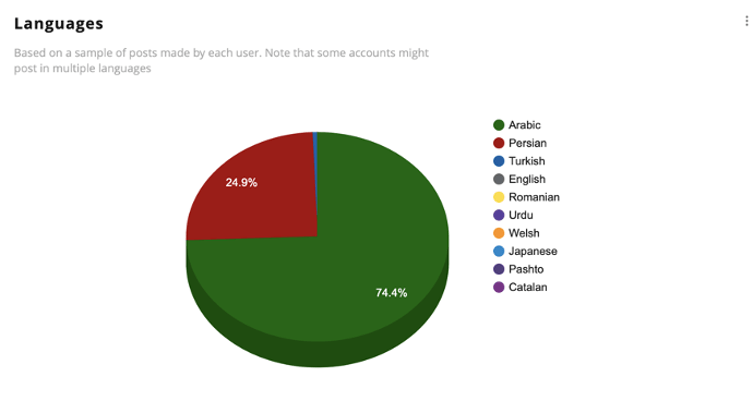
Some users, residing in seemingly unrelated countries like India or South Korea, joined the discourse. Possible explanation? Iraqis living abroad, the use of bots and the cloak of virtual private networks, which obscure geographical boundaries in the digital realm.

Along with the hashtags, fabricated stories, crafted to support the Iranian narrative, flooded social media feeds. But upon closer inspection, many of the claims used fabricated evidence.

Take, for instance, an Instagram-style post purportedly from Al Jazeera, depicting an emergency Israeli National Security Council meeting in response to Iranian strikes. However, the Al Jazeera channel never broadcast such a news item or anything similar. The post was a cleverly disguised forgery.

Similarly, images circulated portraying Kurdish businessman Peshraw Dizayee in the company of security forces, Mossad agents and a rabbi. Yet, meticulous investigations debunked these as digitally altered fabrications .

Even videos, ostensibly showcasing American consulate defenses in Erbil, proved to be recycled footage from an unrelated incident in 2022. The misappropriation of content served to perpetuate false narratives, muddying the waters of truth.

In the era of digital information overload, discerning fact from fiction has become an arduous task. The bombing of Erbil serves as a stark reminder of the dangers lurking in the virtual realm, where misinformation can proliferate unchecked, shaping perceptions and driving agendas.

Opinion | Wall Street Journal marks one year of reporter’s detainment in Russian jail

Evan Gershkovich was arrested a year ago today in Russia while on a reporting assignment for the Journal

A Baltimore bridge collapsed in the middle of the night and two metro newsrooms leapt into action

Coverage from The Baltimore Sun and The Baltimore Banner had much in common but with some marked differences — especially in visuals.

Private equity reporting grants show good return

Projects in Hawaii, Milwaukee and south central Indiana knit news organizations into community life

Opinion | How misinformation will be gender-based in Ghana’s upcoming elections

Fact-checkers must be on the lookout for narratives that target and diminish women candidates

You must be logged in to post a comment.

This site uses Akismet to reduce spam. Learn how your comment data is processed .

Start your day informed and inspired.

Get the Poynter newsletter that's right for you.

More From Forbes

How To Get A Grant For Your Small Business

• Share to Facebook
• Share to Twitter
• Share to Linkedin

Seeking out grant funding is an often untapped opportunity in the entrepreneurial world. While there are complexities involved in the application process, the benefits of obtaining grant money for your small business are potentially vast—ranging from funding for starting a new venture to ramping up your company’s growth.

Small business owners often miss out on opportunities because they feel like the application process is just too cumbersome. Other times, it's because they believe they won't be eligible for a grant. But wouldn't it be a shame to miss out on assistance that could make all the difference?

Take some time to do the research and see what grants and resources are available to you. Chances are, there are programs out there that you qualify for, and with a little effort, you could be on your way to receiving the help you need to take your business to the next level.

Grants vs. Loans and Other Funding

It’s important to note that a grant is not a business loan , and as such, it does not require repayment or equity transfer. Grants consist of funds distributed for a specific purpose, typically defined by the grant program, such as research, community development, or economic expansion. This monetary gift represents a compelling reason for entrepreneurs to pursue grants as part of their financial strategy—it’s essentially free money to grow your business.

Eligibility Criteria for Small Business Grants

Grant eligibility criteria vary widely depending on the provider and the nature of the grant. However, certain common elements typically form part of the eligibility requirements. These might include factors such as location, the industry or sector your business operates within, the number of employees, the type of business entity, and your business’s financial health.

Trump Again Targets Judge s Daughter In New York Criminal Case

Is godzilla x kong the new empire too scary for kids, shai gilgeous-alexander’s quad injury could impact close to thunder’s season.

Common eligibility requirements:

• Business size and legal structure
• Business location and operation domain
• Business industry or niche
• Project or program specifics
• Financial needs and plan

Preparing a Compelling Small Business Grant Application

Crafting a successful grant proposal is a multi-step process that requires a strategic approach. Remember, competition for grants is often fierce, and a well-prepared proposal is your key to standing out.

A standard grant proposal includes the following sections:

Business overview and mission: Clearly outline your business’s mission and the purpose of the grant request within this context.

Project description: Define your project’s goals, scope, and anticipated outcomes, showing how the grant will support these initiatives.

Budget and financing plan: Lay out a detailed budget illustrating how the grant money will be used to achieve the project’s objectives.

Impact and benefit analysis: Articulate the broader impact and potential benefits your project will have on the community, industry, or economy, in alignment with the grantor’s mission.

Sustainability plan: Detail how the positive impacts of the project will continue beyond the grant period, ensuring lasting value.

Navigating the Application Process

Each grantor will have specific application guidelines that you must follow meticulously. This typically involves completing an application form, attaching required documents, and submitting the proposal within a given timeframe. Be mindful of deadlines and consider starting the application well in advance to avoid rushing the process.

Writing a Persuasive Grant Proposal

When writing your grant proposal , focus on addressing the funder’s key concerns, showcasing a clear alignment between your business’s activities and the grantor’s mission, and compelling storytelling that highlights the impact of your intended project. Data-driven arguments and evidence of past success can also bolster your proposal.

Overcoming Common Obstacles in the Grant Application Journey

Even with diligent preparation, the road to securing a grant can be fraught with obstacles. Being aware of these challenges and knowing how to overcome them is crucial to your success.

Establishing a solid business case

Grant providers are looking to support initiatives that have a strong likelihood of success. This means you must demonstrate the viability of your business and the project, complete with a strategic plan, market research, and any relevant track record your team has.

Articulating the right message

Effective communication with the grantor requires you to tailor your pitch to their preferences, priorities, and language. Engaging with the grantor prior to the application can provide valuable insights on how to properly frame your proposal.

Managing the application volume

Applying for multiple grants can be a time-consuming process. In such cases, consider establishing a system for managing the application process, including a calendar with important dates, reusable templates, and a clear distribution of tasks among team members or partners.

The bottom line is that the world of small business grants is rich with opportunities for ambitious entrepreneurs willing to invest the time and effort in this pursuit. By understanding the nuances of the grant application process, aligning your business goals with potential funding sources, and maintaining a strategic approach to securing and deploying grant money, you can position your venture for growth and success.

Melissa Houston, CPA is the author of Cash Confident: An Entrepreneur’s Guide to Creating a Profitable Business . She is the founder of She Means Profit, which is a podcast and blog . As a Finance Strategist for small business owners, Melissa helps successful business owners increase their profit margins so that they keep more money in their pocket and increase their net worth.

The opinions expressed in this article are not intended to replace any professional or expert accounting and/or tax advice whatsoever.

• Editorial Standards
• Reprints & Permissions

• 0 Shopping Cart

The Somerset Levels Flood Case Study

The Somerset Levels are a coastal plain and wetland area in Somerset, England. Thousands of years ago, the area was covered by the sea, but today it’s a landscape of rivers and wetlands – artificially drained, irrigated and modified to allow productive farming.

It is claimed that the Somerset Levels are one of the lowest areas in the UK. This is because much of the area lies below the high-water mark of spring tides. The area is very flat and has a maximum altitude of 8m above sea level. All rivers in this area, including Axe, Sheppey and Brue, are in the north, while to the south, the rivers the Cary, Yeo, Tone and Parrett drain into the Bristol Channel.

In January 2014, the Somerset Levels experienced floods greater than any other in living memory. Estimates suggest that 10% of the area was underwater when the flooding was greatest.

Somerset Levels 2014 flood map

What were the physical causes of flooding in the Somerset Levels?

A quick succession of prolonged Atlantic storms, with persistent rainfall and gale-force winds, was the primary cause of flooding. The rivers could not cope with the significant amount of rain that fell. High tides in the Bristol Channel and its narrowing also create tidal surges. These blocked the floodwater, trying to escape the Somerset Levels. Coastal defences coped with the tidal surges.

What were the human causes of flooding in the Somerset Levels?

There had been less dredging of the river channels on the Somerset Levels leading up to 2014. However, as a result, the channels had risen due to sediment accumulation. This reduced the capacity of rivers to transport water, leading to flooding.

Change in farming practices has also contributed to flooding. Much of the land has been converted from grassland to grow maise. This more intensive use of the land means it is less able to retain water, causing it to run over the surface rather than being absorbed.

What were the impacts of flooding in the Somerset Levels?

The flood was the most significant hazard to affect this area ever. The event was so significant it dominated the national news coverage.

The flooding had a range of social, economic and environmental impacts.

What were the social impacts of the Somerset Levels floods?

Over 600 homes and 16 farms were evacuated, resulting in many people requiring temporary accommodation, where many stayed for several months. In addition, several villages, such as Moorland and Muchelney, were cut off after roads were flooded. Power supplies were cut off during a time when temperatures were low.

What were the economic impacts of the Somerset Levels floods?

Somerset County Council estimates that the cost of flood damage was over £10 million. The agricultural industry was among the hardest hit, with over fourteen thousand hectares of agricultural land used for crops and grazing flooded for three to four weeks. One thousand livestock were evacuated from the affected farms.

Many main roads were closed, including the A361 linking Taunton and Street. Flooding disrupted train services on the main Bristol line between Taunton and Bridgwater.

Fuel used to power emergency pumps cost £200 000 per week. An estimated £1 million was lost by local businesses. The Somerset floods cost the county’s tourism industry an estimated £200 million.

There were several incidents of crime during the floods. Nine hundred litres of fuel was stolen from a pumping station in Westonzoyland. There were also reports of heating oil and quad bikes being stolen from homes affected by flooding.

Insurance costs increased in flood-hit areas of Somerset.

What were the environmental impacts of the Somerset Levels floods?

The environmental impact included the extensive contamination of floodwaters by sewage, oil, and various chemical pollutants. Following the recession of floodwaters, a significant amount of debris required clearing, while stagnant water accumulated over several months needed to be re-oxygenated before reintroduction into rivers. Failure to do so would have caused substantial harm to marine ecosystems.

The soil was damaged after being underwater for nearly three months. In some areas, it took over two years to restore the soil before crops could be grown.

Immediate response to the Somerset Levels flood

As expected for a high-income country (HIC), the response to the flood was well-organised and rapid.

Local people in South West England were warned of heavy rain when the Met Office issued an amber warning. The public was advised to prepare for significant flooding by the Environmental Agency. Many people used sandbags to protect their property and moved valuable items upstairs. In Moorland, a man constructed a large wall out of clay and mud to protect his house from flooding.

Rescue boats were used to help stranded people by the fire brigade who also visited hundreds of properties. Rescue crews supported residents of Moorland in evacuating. The owners of some 80 homes agreed to evacuate; however, around 30 residents stayed at home. Additional police patrols were introduced as a result of increased crime.

The army was sent into the area with specialist equipment towards the end of January. They issued sandbags and distributed food. 40 Royal Marines later joined them to provide additional support.

Sixty-five pumps were used to drain 65 million m3 of floodwater.

Local people, led by the Flooding on the Levels Action Group (FLAG), provided local support to the people affected. This included fundraising and the collection and distribution of food. They also used social media, such as Facebook and Twitter, to share the news.

The government made an estimated £15m to meet the immediate costs of protecting lives and properties.

Long-term response to the Somerset Levels flood

The long-term response to the Somerset Levels flood focussed on management techniques to reduce the risk of future floods. As a result, the Somerset Levels and Moors Action Plan was developed and included measures such as reintroducing dredging, constructing a tidal barrage and additional permanent pumping stations. The scheme is part of a 20-year plan for the Somerset Levels and will total £100 million.

Premium Resources

Please support internet geography.

If you've found the resources on this page useful please consider making a secure donation via PayPal to support the development of the site. The site is self-funded and your support is really appreciated.

Related Topics

Use the images below to explore related GeoTopics.

Topic Home

Next topic page, share this:.

• Click to share on Twitter (Opens in new window)
• Click to share on Facebook (Opens in new window)
• Click to share on Pinterest (Opens in new window)
• Click to email a link to a friend (Opens in new window)
• Click to share on WhatsApp (Opens in new window)
• Click to print (Opens in new window)

If you've found the resources on this site useful please consider making a secure donation via PayPal to support the development of the site. The site is self-funded and your support is really appreciated.

Search Internet Geography

Top posts and pages.

Latest Blog Entries

Pin It on Pinterest

• Click to share
• Print Friendly

Advertisement

Supported by

Eclipses Injured Their Eyes, and the World Never Looked the Same

A number of case studies published after recent total solar eclipses highlight the importance of safe viewing.

• Share full article

By Gina Kolata

This article is part of The Times’s coverage of the April 8 eclipse , the last time a total solar eclipse will be visible in most of North America for 20 years.

A young woman visited New York Eye & Ear Infirmary of Mount Sinai Hospital shortly after the eclipse of Aug. 21, 2017. She told Dr. Avnish Deobhakta, an ophthalmologist, that she had a black area in her vision, and then drew a crescent shape for him on a piece of paper.

When Dr. Deobhakta examined her eyes, he was astonished. He saw a burn on her retina that was exactly the same shape. It was “almost like a branding,” he said.

She had looked at the sun during the eclipse without any protection. The burn was an image of the sun’s outer edge.

With every eclipse, ophthalmologists see patients who looked at the sun and complain afterward that their vision is distorted: They see small black spots, their eyes are watery and sensitive to light. Usually, the symptoms resolve, although it may take several weeks to a year.

But the woman’s retinal burns, which Dr. Deobhakta and colleagues described in a medical case write-up, would not heal. Her retina was permanently scarred and a sign of the severity of injuries that can follow looking at an eclipse without proper precautions.

With the coming eclipse in April, ophthalmologists advise people to be careful and not assume that short glances at the sun are safe. Damage can occur, they say, in less than a minute.

David Calkins, director of the Vanderbilt Vision Research Center and vice chair of the Vanderbilt Eye Institute in Nashville, said younger people were most at risk of retinal injury, possibly because the lens of their eye is clearer than the lens in older people. He said they also may be a bit more reckless.

But age is no guarantee of safe eclipse viewing.

A study described 20 people aged 15 to 82 in England who complained of symptoms like black spots in their vision or blurry vision after an eclipse in 1999. Four said they used eclipse glasses; one said she used sunglasses. The rest looked with naked eyes.

Five had visible damage to their retinas. All but four of the 20 were better after seven months.

Not everyone is so lucky. A study published last year involved four young Irish women who looked at the sun during a religious gathering in October 2009 . The women, who did not know one another, sought medical attention within a few days of looking at the sun. They complained of blind spots in the center of their vision and said objects appeared distorted and blurred.

Investigators from Galway University Hospital followed up with the women for an average of more than five years. One was followed for 11 years.

Years later, the researchers reported, all of the women still had the blind spots.

For Dr. Deobhakta, the situation with the woman in 2017 is a cautionary tale.

While she did put on protective glasses for part of her viewing of the eclipse, she at first looked at it several times for about six seconds each time without protection.

She felt fine for four hours. Then her symptoms emerged: blurred vision, distorted shapes and colors, and that crescent-shaped black spot in the center of her vision with her left eye.

Most people look at an eclipse through special eclipse glasses. Often the glasses have a cardboard body with special film in the eyeholes that filters out harmful rays.

Dr. Deobhakta said he did not trust many of the eclipse glasses being sold and felt it was not worth taking a chance on them. He prefers an indirect method that involves using pinholes, like in a colander, to cast the sun’s shadow on the ground.

Professional groups say many eclipse glasses are safe but urge caution when buying them. The American Astronomical Society reported that potentially unsafe eclipse glasses flooded the market before the 2017 eclipse.

To help people find eclipse glasses, the astronomical society lists reliable sellers and distributors.

Legitimate eclipse glasses must meet specific international safety standards known as ISO 12312-2. Testing requires a spectrophotometer that measures how much ultraviolet, visible and infrared light gets through the glasses.

But an ISO logo on the glasses is not necessarily an assurance, the astronomical society warns, because dealers can — and some do — snatch an ISO logo from the internet and put it on their glasses.

Rick Fienberg, project manager of the astronomical society’s Solar Eclipse Task Force, said counterfeiting companies were also putting the names of legitimate distributors on their products. That doesn’t necessarily mean they’re unsafe, he added. But it does mean that the seller, or the company that sold it the products, is committing fraud.

Dr. Fienberg suggests buying directly from a seller on the astronomical society’s list.

But, he said, if you are worried about your glasses, there is a way to see if they are effective. Look around a room with the eclipse glasses on. The glasses should be so dark you can’t see anything. Then, go outside and glance at the sun with the glasses on. You probably are safe, he said, if you can see the sun through the lenses and “the image is sharp and comfortably bright.”

Dr. Deobhakta still worries. He says he knows he is overly cautious but can’t help warning people about the coming eclipse.

“Do not look at it whether you have glasses or not,” he said. “I’m not going to let my family members look at it. I’m a doctor. That’s why I say what I say. I saw what happened.”

An earlier version of this article, using information from a doctor, misstated the source of a woman’s eye injury. She looked at the sun’s outer edge, not its corona.

How we handle corrections

Gina Kolata reports on diseases and treatments, how treatments are discovered and tested, and how they affect people. More about Gina Kolata