relative income hypothesis graph

Relative Income Hypothesis

Post author: Viren Rehal
Post published: August 17, 2022
Post category: Consumption function / Macroeconomics
Post comments: 0 Comments

Duesenberry took a different approach to develop a model explaining consumption behaviour. While other models such as the permanent income hypothesis are based on utility function independent of consumption by other individuals, this model considers utility as a function of relative consumption. That is, utility is maximized by considering the consumption levels of the rest of the population. Hence, it is known as the Relative Income Hypothesis.

utility function and relative consumption

According to Duesenberry, consumers are not concerned about absolute consumption. But, their consumption decisions are based on relative consumption in comparison to the rest of the population. Generally, utility is a function of the absolute quantity of goods (absolute consumption). However, relative income hypothesis proposes a slightly different utility function which can be stated as follows:

According to this utility function, there is a positive relationship between utility and relative consumption. This means that utility will increase when consumption increases relative to the average consumption of the population. Or, when the increase in consumption is greater than the increase in the average consumption of the population.

This approach can explain both cross-sectional and long-run behaviour of consumption observed in empirical studies:

MPC<APC across cross-sections

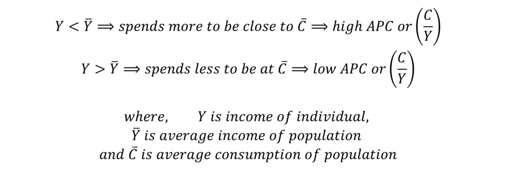
The above utility function implies that consumption decisions depend on income distribution in the economy. When a consumer has below-average income, he will try to match the average consumption level of the population. They will end up spending a larger proportion of their below-average income. As a result, APC (C / Y) will be high in the case of individuals with lower than average income. On the other hand, individuals with income higher than the average population income will spend a lower proportion of income on consumption because they can match average consumption by spending a lesser portion of income. Hence, high-income groups will have lower APC (C / Y).

With APC falling with higher income, MPC will be less than APC (MPC<APC) across different sections which explains consumption behaviour observed in cross-sectional studies.

MPC = APC in the long run

The economy will grow along the trend in the long run. With growth, the income of consumers will increase, however, the average income of the population will also increase along with it. Hence, relative income will still remain stable even with rising incomes because the income of the entire population increases which also shifts average income upwards.

Since relative income is still stable, there is no reason for the APC (C / Y) to change. It will remain constant as the economy grows along the trend line. As long as the relative distribution of income is stable, this hypothesis will hold true because growth in the economy will lead to a proportionate growth in consumption for all individuals.

Present consumption, past consumption and cyclical fluctuations

According to Duesenberry, past consumption also affects present consumption. Therefore, consumption in previous time periods along with current relative income help in determining current consumption. For individuals, it is difficult to reduce consumption in the current period after attaining a certain level of consumption in the previous time periods. It is easier for them to reduce their savings instead of consumption.

Duesenberry formulated this in terms of savings. It suggests that the savings to income ratio depend on the level of current income in comparison to the previous peak income (which is the highest previous period income). This relationship can be expressed as follows:

There is a positive relationship between the saving-income ratio and relative income. A rise in income relative to previous peak income leads to an increase in the saving-income ratio. Therefore, the proportion of savings increases with an increase in income relative to peak income. This savings function can be easily converted into a consumption function as follows:

As income grows along a trend over a long period of time, the previous peak income will always be the income from the previous year’s income. As a result, an increase in the ratio of income to peak income will be equal to the growth of the economy along the trend. If the economy grows by 5 per cent, this ratio will increase by 5 per cent as well. Hence, the ACP will be constant along the trend.

Cyclical fluctuations

Although ACP is constant along the trend growth, there are cyclical fluctuations around this trend due to business cycles. The ACP (C / Y) has a negative relationship with income because the coefficient (beta 2 ) is negative.

The above equation can be used to estimate MPC:

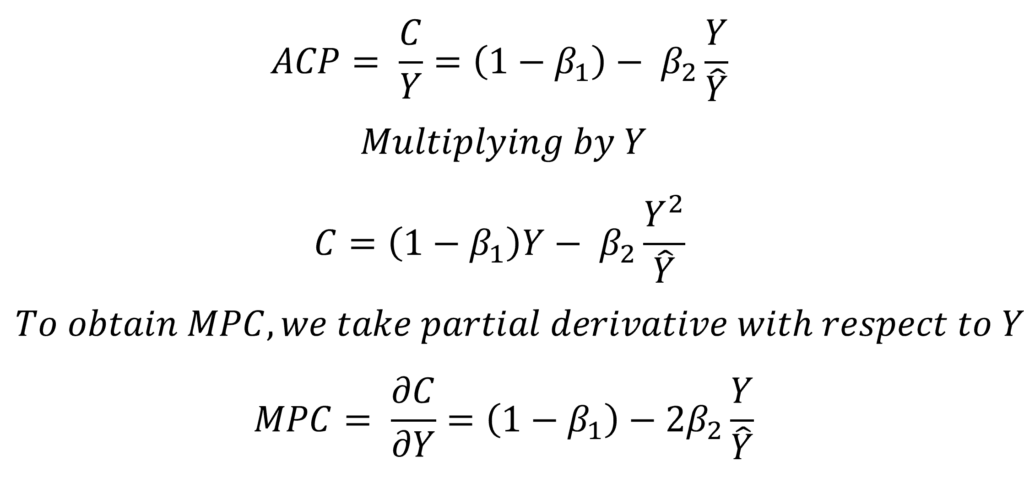
If we compare both equations of APC and MPC, it is clear that MPC<APC. When the peak income is fixed, the MPC equation has a greater negative component as it multiplies the negative component by 2.

Therefore, we can conclude that MPC<APC in the shorter periods of business cycles when the APC falls with an increase in income. In the long run, however, APC is constant with growth along the trend.

the ratchet effect

The combination of short-run and long-run consumption explained by the relative income hypothesis gives us the ratchet effect. In the long run, the economy grows along the trend line shown by the long-run consumption function. The APC is constant in the long run. This means that the proportion of income spent on consumption remains constant because relative income is stable.

However, if the economy falls into recession and income decreases, short-run consumption moves on to consumption functions shown by C A and C B . On these short-run curves, APC falls as income rises during the recovery period till it reaches the long-run function or the trend. At that point, growth resumes at its constant APC after reaching the previous peak period of income. The MPC on these short-run curves can be estimated using the above equations and it will always be less than APC on the short-run curves C A and C B .

Criticism of Relative Income Hypothesis

The role of wealth or assets is not taken into consideration in the relative income hypothesis. But, wealth plays an important role in determining consumption levels. Although this theory provides a different perspective through relative income, theories such as the permanent income hypothesis and life cycle hypothesis are usually preferred because of their incorporation of wealth into consumption behaviour. In the permanent income hypothesis, the role of wealth is implicitly taken. But, the life cycle hypothesis explicitly states the role of assets and wealth.

Permanent income hypothesis, accelerator theory and its process, phillips curve: short run and long run, leave a reply cancel reply.

To provide the best experiences, we and our partners use technologies like cookies to store and/or access device information. Consenting to these technologies will allow us and our partners to process personal data such as browsing behavior or unique IDs on this site and show (non-) personalized ads. Not consenting or withdrawing consent, may adversely affect certain features and functions.

Click below to consent to the above or make granular choices. Your choices will be applied to this site only. You can change your settings at any time, including withdrawing your consent, by using the toggles on the Cookie Policy, or by clicking on the manage consent button at the bottom of the screen.

Publication: The Relative Income and Relative Deprivation Hypotheses : A Review of the Empirical Literature

Files in English

Link to data set, report series, other publications in this report series.

Publication Climate Shocks and the Poor ( Washington, DC: World Bank , 2024-03-29 ) Triyana, Margaret ; Jiang, Andy Weicheng ; Hu, Yurui ; Naoaj, MD Shah Show more There is a rapidly growing literature on the link between climate change and poverty. This study reviews the existing literature on whether the poor are more exposed to climate shocks and whether they are more adversely affected. About two-thirds of the studies in our analyzed sample find that the poor are more exposed to climate shocks than is the rest of the population and four-fifths of the studies find that the poor are more adversely affected by climate shocks than is the rest of the population. Income and human capital losses tend to be concentrated among the poor. These findings highlight the potential long-term risk of a climate-change induced poverty trap and the need for targeted interventions to protect the poor from the adverse effects of climate shocks. Show more
Publication How Delayed Learning about Climate Uncertainty Impacts Decarbonization Investment Strategies ( Washington, DC: World Bank , 2024-03-29 ) Bauer, Adam Michael ; McIsaac, Florent ; Hallegatte, Stéphane ; Hallegatte, Stéphane Show more The Paris Agreement established that global warming should be limited to “well below” 2◦C and encouraged efforts to limit warming to 1.5◦C. Achieving this goal presents a significant challenge, especially given the presence of (i) economic inertia and adjustment costs, which penalize a swift transition away from fossil fuels, and (ii) climate uncertainty that, for example, hinders the ability to predict the amount of emissions that can be emitted before a given temperature target is passed, which is often referred to as the remaining carbon budget. This paper presents a modeling framework that explores optimal decarbonization investment strategy when both delayed learning about the remaining carbon budget and adjustment costs are present. The findings show that delaying learning about the remaining carbon budget impacts investment in three ways: (i) the cost of policy increases, especially when adjustment costs are present; (ii) abatement investment is front-loaded relative to the certainty policy; and (iii) the sectoral allocation of investment changes to favor declining investment pathways rather than bell-shaped paths. The latter effect is especially pronounced in hard-to-abate sectors, such as heavy industry. Each of the effects can be traced back to the carbon price distribution inheriting a “heavy tail” when the remaining carbon budget is learned later in the century. The paper highlights how climate uncertainty and adjustment costs combined result in a more aggressive least-cost strategy for decarbonization investment. Show more
Publication The Sovereign Spread Compressing Effect of Fiscal Rules during Global Crises ( Washington, DC: World Bank , 2024-03-28 ) Islamaj, Ergys ; Samano Penaloza, Agustin ; Sommers, Scott Show more Do fiscal rules help suppress sovereign spreads during periods of global financial stress Yes! This paper examines whether fiscal rules contribute to mitigating sovereign spreads in emerging markets and developing economies during periods of heightened financial and economic volatility worldwide. It finds that the presence of fiscal rules is statistically significantly associated with lower sovereign spreads during the COVID-19 crisis — about 350 basis points lower on average. Interestingly, this correlation persists even when nations deviate from these rules, indicating an expectation of post-crisis compliance. The study shows that deviations from fiscal rules are typically short-lived, with fiscal balance rules reinstated within 3.5 years. Robustness checks, including controls for institutional quality, fiscal rule strength, and global and regional factors confirm these results. Overall, the findings suggest that fiscal rules can help emerging markets and developing economies signal fiscal responsibility during episodes of global financial stress, reducing borrowing costs relative to countries without fiscal rules. Show more
Publication The Macroeconomic Impact of Climate Shocks in Uruguay ( Washington, DC: World Bank , 2024-03-27 ) Giuliano, Fernando ; Navia, Daniel ; Ruberl, Heather Show more Uruguay is an economy that is vulnerable to precipitation patterns, as evidenced during the country’s historic 2022/23 drought. Yet, and despite its rich macroeconomic and climate data environment, the country does not have a consistent macroeconomic model to address the aggregate impact of climate shocks, let alone the expected additional impact from climate change. This paper intends to fill this gap by integrating climate shocks into the World Bank’s Macro-Fiscal Model, its workhorse structural macroeconomic projection model. Building on existing country studies on the sectoral effects of droughts and floods, the analysis finds that the volatility of a simulated Uruguayan economy only subject to historical climate shocks reaches 22 percent of the historical volatility of gross domestic product. Moreover, as climate shocks are only one of many shocks that can simultaneously affect an economy, incorporating exogenous macroeconomic shocks into historical climate shocks exacerbates volatility and increases potential losses. Gross domestic product can fall by 2.3 percent under a combined negative climate and macroeconomic shock of the type witnessed once every six years on average, and 4.1 percent under a once-in-40-years combined negative shock. Climate change compounds these effects going forward, worsening the magnitude of the downside risks from droughts by between 18 and 30 percent, although estimates incorporating climate change are subject to large uncertainty. The order of magnitude of these effects calls for a more systematic consideration of climate shocks in macroeconomic projections and fiscal risk assessments for Uruguay. Show more
Publication The Role of Firm Dynamics in Aggregate Productivity, Job Flows, and Wage Inequality in Ecuador ( Washington, DC: World Bank , 2024-03-27 ) Patiño Peña, Fausto ; Ferro, Esteban Show more This paper examines the role of firm dynamics in aggregate total factor productivity, job flows, and wage inequality in Ecuador. Utilizing a comprehensive employer-employee dataset, the paper documents firm dynamics and job flow patterns that are consistent with the presence of market distortions. Also, the paper identifies factor misallocation as the main contributor to Ecuador's total factor productivity deceleration. Given these trends, the paper explores allocative inefficiency drivers through firm- and industry-level regressions. Firms in the top productivity quintile face distortive non-wage labor costs that are 3.7 times higher than the bottom quintile, after controlling for firm size and age. The findings also provide evidence of credit misallocation across firms. Additionally, industries with higher job mobility, credit access, and competition and lower non-wage labor costs, minimum wage incidence, and zombie firms demonstrate higher allocative efficiency. Moreover, worker-level regressions indicate that misallocation drivers explain up to 41 percent of wage inequality, with non-wage labor costs and product market frictions as distortions driving this inequality. Show more

Journal Volume

Journal issue, collections, associated urls, associated content.

Macroeconomics: Theory and Policy by Vanita Agarwal

Get full access to Macroeconomics: Theory and Policy and 60K+ other titles, with a free 10-day trial of O'Reilly.

There are also live events, courses curated by job role, and more.

Theories of Consumption

After studying this topic, you should be able to understand

The basic principle of absolute income hypothesis is that the individual consumer will determine the fraction of his current income that he will allocate to consumption on the basis of his absolute income level.
According to the relative income hypothesis, the fraction of a family’s income that will be allocated to consumption will depend on its income level relative to the income level of the other families with which it classifies itself .
The permanent income hypothesis puts forward the view that consumption is related to the permanent income .
The average propensity to consume, expressed in terms of the permanent income, is the same on an average for all ...

Get Macroeconomics: Theory and Policy now with the O’Reilly learning platform.

O’Reilly members experience books, live events, courses curated by job role, and more from O’Reilly and nearly 200 top publishers.

Don’t leave empty-handed

Get Mark Richards’s Software Architecture Patterns ebook to better understand how to design components—and how they should interact.

It’s yours, free.

Check it out now on O’Reilly

Dive in for free with a 10-day trial of the O’Reilly learning platform—then explore all the other resources our members count on to build skills and solve problems every day.

Subscriber Services
For Authors
Publications
Archaeology
Art & Architecture
Bilingual dictionaries
Classical studies
Encyclopedias
English Dictionaries and Thesauri
Language reference
Linguistics
Media studies
Medicine and health
Names studies
Performing arts
Science and technology
Social sciences
Society and culture
Overview Pages
Subject Reference
English Dictionaries
Bilingual Dictionaries

More Like This

Show all results sharing these subjects:

relative income hypothesis

Quick reference.

The theory that savings behaviour is affected by a person's relative position in the income distribution. Thus at a given level of real income, a person may be a relatively poor member of a rich community, or a relatively rich member of a poor community. The member of the richer community is expected to consume more and save less, as ideas of what constitutes a socially acceptable minimum level of consumption are influenced by what is habitual to their friends and neighbours. This analysis also applies to comparisons between different countries or regions, or the same country at different times.

From: relative income hypothesis in A Dictionary of Economics »

Subjects: Social sciences — Economics

An Influence of Relative Income on the Marginal Propensity to Consume: Evidence from Shanghai

Reviewed: 09 November 2016 Published: 01 February 2017

DOI: 10.5772/66785

Cite this chapter

There are two ways to cite this chapter:

From the Proceeding

Proceedings of the 2nd Czech-China Scientific Conference 2016

Edited by Jaromir Gottvald and Petr Praus

To purchase hard copies of this book, please contact the representative in India: CBS Publishers & Distributors Pvt. Ltd. www.cbspd.com | [email protected]

Chapter metrics overview

1,693 Chapter Downloads

Impact of this chapter

Total Chapter Downloads on intechopen.com

Total Chapter Views on intechopen.com

Overall attention for this chapters

This chapter deals with the question whether there is a relationship between the marginal propensity to consume and the status of the household in income distribution represented by a relative income. If so, then the current assumption of mainstream theory of consumption about the constant marginal propensity to consume could no longer be considered realistic and it will be necessary to take the element of relative income as a new key determinant of general consumption function. The aim of this work is to identify, describe, and prove an influence of relative income on the marginal propensity to consume using data for urban residents of Shanghai and to prove the correctness of Duesenberry’s relative income hypothesis. To achieve this goal, we use a panel regression, through which the results clearly confirm the validity of the initial hypothesis about the existence of functional dependence of the marginal propensity to consume on the relative income and so it fully supports the idea of interdependent concept of utility and consumption.

relative income
marginal propensity to consume
Duesenberry’s hypothesis
interdependent utility
consumption function

Author Information

Ondřej badura *.

Shijiazhuang University of Economics, East HuaiAn Road, Shijiazhuang, Hebei, China

Tomáš Wroblowský

*Address all correspondence to: [email protected]

JEL : D11, D12

1. Introduction

Consumption represents a key determinant of economic thought in many ways, not so much for its immense practical significance, but rather because it de facto represents the essence of economics itself, the essence of the issue of infinite needs and finite resources. Both in terms of microeconomics, that consumption hypotheses are always necessarily based on, and within a macroeconomic approach the widely accepted theory of consumption of mainstream economics seems to be very well formulated and developed and as such it has remained virtually unaltered for nearly 60 years. But is this theoretical concept entirely accurate and complete? Could not even here be one of the major determinants of the general consumption function omitted? Now these questions are a starting point of this chapter.

Since the 1950s of the twentieth century, the approach of permanent income theory and lifecycle hypothesis has prevailed in professional circles of economic theory. This mainstream view of the basic economic laws determining household consumption is in professional economic texts established to such an extent that the different approaches are practically not visible. However, this does not mean that there are not any alternative hypotheses of consumer behavior. We can find many critical perspectives on the standard theory of consumption, but often it is only a solution of narrowly focused issues, the pieces of a mosaic of complex alternative theory, that as a whole remains fragmented across countless of professional studies as poited out by Ackerman (1997) . And if this comprehensive theory arose after all, still it was ignored for various reasons. And that is exactly also the case of Duesenberry’s relative income hypothesis—consumer concept, based on the idea of interdependent utility, which has the potential with theoretical way to challenge a complete validity of the consumption theory of mainstream economics, and ultimately and primarily to significantly enrich the basic pattern of generally accepted consumption function of life cycle-permanent income hypothesis (LC-PIH) 1 ( Mason, 2000 ).

Income and price are the key determinants of consumer choice as for mainstream economics. Relative income hypothesis, however, points out the fact that if the consumer is also affected by consumption habits of his surroundings, then the income itself must be seen in two ways: in absolute and in relative terms. From these two concepts of the basic economic determinant of general consumption function, it stems also two channels of influence on the total amount of consumption. An absolute concept of income implies a direct effect, already well known from the Keynesian consumption function. Higher disposable income will lead to a proportionately greater amount of consumer spending. A variable of disposable income then figures in the functional form of consumer equation simply as the independent variable directly explaining the level of consumption. While the relative concept of income, at least according to the principles of Duesenberry’s hypothesis, implies an indirect effect. Higher disposable income will lead to higher position of household across income distribution and according to interdependent concept of utility and consumption also to a lower value of the marginal propensity to consume (MPC). The decline of MPC then, as an element transforming disposable income into consumption, negatively affects the ultimate level of consumption. The position of household in income distribution is then represented in the consumption pattern as an independent variable, which indirectly through MPC affects the level of consumption.

The problem is that while the absolute (direct) income effect is a well-known matter and the virtually undisputed, relative (indirect) income effect remains often completely ignored by professional economic communities, whether in the form of Keynesian consumption function or access of LC-PIH. It is true that every relevant and really applicable model must be extracted of elements that have not a major impact on it. However, is also the relative income effect the insignificant element, which should be completely removed out of the consumption function without a trace? Is the interdependent concept of utility from the consumption a matter totally irrelevant? If so, then this whole work is a pointless effort.

To explore this matter, we use data from China, which has been undergoing significant structural changes recently. The shift from investment and export-oriented economy into consumption-oriented economy is one of the biggest changes. Although the consumption contribution to the country’s GDP is still lower than in all developed countries, the change of government’s policy (hence the whole economy) is significant. Such development turns the attention of researchers to the consumption and its determinants.

Unfortunately, only few research studies have been carried out in this field earlier. There are several studies analyzing the factors influencing very low consumption rates in China (see for example Horioka and Wan, 2007 ; Yang et al., 2011 ) or studies generally describing the consumption determinants on the macro level as Guo and Papa (2010) . Many studies also focus on inequality of income distribution as a factor affecting the consumption (see Lou and Li, 2011 ). However, none of these studies mention the relative income as one of the possible consumption determinants. The interdependence of consumers seems to be analyzed much more by marketing specialists, see for example the studies of Zhang and Kim (2013) ; Yu (2014) . These studies can provide useful insight into the relations among the consumers, but they cannot provide any evidence of the influence of “keeping up with the Joneses” effect on the final general consumption function.

The aim of this work is to identify, describe, and prove an influence of relative income on the marginal propensity to consume using data of urban residents of Shanghai and thus to prove the correctness of Duesenberry’s hypothesis.

2. Relative income hypothesis

“Professor Duesenberry’s study of the impact of budgetary and aggregative empirical consumption data on the received theory of consumer behavior is one of the most significant contributions of the postwar period to our understanding of economic behavior" written in his review by Arrow (1950 , p. 906), his time respected neoclassical economist and later Nobel prize laureate in economics.

The relative income hypothesis is fundamentally built on criticism of established neoclassical preconditions for the creation of demand and Keynesian theory of consumption based on them. The main and fundamental idea with which Duesenberry (1949) comes to the field of knowledge in order to confront these established relationships of mainstream economics is a complex social concept of consumer and revision of Veblen’s demonstration effect ( Veblen, 1899 ), which the author gives a particular dimension through income distribution of households.

We can find two fundamental propositions in the work of James Duesenberry, let's say postulates, on which the theory of relative income stands and which are the basis for its further implications ( Palley, 2010 , p. 6):

“The strength of any individual’s desire to increase his consumption expenditure is a function of the ratio of his expenditure to some weighted average of the expenditures of others with whom he comes into contact.”

“The fundamental psychological postulate underlying our argument is that it is harder for a family to reduce its expenditure from a higher level than for a family to refrain from making high expenditures in the first place.”

The real foundation of the new model is, however, the first claim. The author himself called this effect as keeping up with the Joneses or the effect of relative income. The principle is mainly simple. The consumer is not isolated from others, he lives in a world where he every day meets his friends, colleagues, family, his neighbors, and so on. And not only he meets them, especially he is confronted with their consumption. He sees what they buy, what they spend for, by what they form their standard of living, and their position in society. He sees what Veblen saw in his theory, the so-called pompous ("pointless") consumption. Unlike Veblen (1899) , for the majority of the population, these consumer expenditures are not pointless, because it allows them to reach the intangible social values—a status. And that is what this is about. Our consumer shall see how people around him buy goods for their ceremonial value, before his eyes they increase the value of their status, strengthen their social position and even he does not want to be left behind. Therefore, if the consumer belongs to low-income households (his disposable income ( Y D ) is under the society-wide weighted average ( Y ¯ D )), then he spends more of his disposable income just to demonstrate that he can afford it, just to catch up with social status of others. His MPC is then relatively high. Conversely, high-income households 2 (whose Y D is above the society-wide weighted average) usually already have valuable status, therefore they have not such a motivation to "catch up with someone", they do not have to spend so much of their income and vice versa they save more, simply because they can afford it. So we come to the first simple implication:

where the higher value of the index n stands for a household with a higher value of relative disposable income ( Y RD ), most simply expressed as:

Put simply marginal propensity to consume can be written as a negative functional dependence of relative (disposable) income, as similarly shows ( Palley, 2010 ):

The total amount of household consumption C is then given by the product of disposable income and the marginal propensity to consume, which is not constant now (as naively assumes the mainstream theory of consumption), but it depends on the position of the entity in the curve of income distribution:

Plain view on the derivation of the final rule of general consumption function, especially on the relationship between MPC and Y RD (Eq.( 3 )), can logically evoke questions like: Is not such a general notation too trivial? Would it be possible at this point to express the dependence of marginal propensity to consume on relative disposable income in particular functional form? We find in the later part of this work that the real version of this relationship is not such a trivial matter, it depends on the number of other factors and it simply cannot be expressed in the general shape like this. There are only a number of methods by which this relationship can be approximated into particular form. One of these ways is, as we could see, the central theme of this work.

3. Methods and data

The first thing we need to realize at this point is that the marginal propensity to consume of households does not change due to the amount of disposable income, but depending on the relative disposable income, as shown in Eq. ( 3 ).This is essentially a central idea of discussed hypothesis, a key contribution to the debate on the form of consumption function. As literally written by Alvarez-Cuadrado and Long (2011 , p. 1489): "For any given relative income distribution, the percentage of income saved by a family will tend to be unique, invariant, and increasing function of its percentile position in the income distribution. The percentage saved will be independent of the absolute level of income. It follows that the aggregate saving ratio will be independent of the absolute level of income." An important factor is that although the MPC and therefore also APC of households differ substantially across the Lorenz curve of distribution of disposable income (which we can figure out even with simplest common sense, but no longer with the standard theory of consumption), it is this way only because of the effect of relative income, which does not exist at the aggregate level. 3 Average propensity to consume for the whole economy is then constant in the long term, thus the relative income hypothesis is entirely consistent with the observation presented by Kuznets et al. (1946) 4 70 years ago.

Whatever is the strength of the effect of relative income throughout income distribution in the society, the MPC for every household, more precisely a category to which the household belongs, is always given by a functional relationship due to its relative disposable income. And as it is well known that the function generates for any given situation only one result, therefore, each type of household also has only one marginal propensity to consume. Maybe the above sounds trivial and like a commonplace, but it is important to realize that the MPC of different groups of households does not change over time ceteris paribus, 5 it is independent on the absolute amount of income and so it has for each Y D a constant value. But first and foremost, as the previous lines try to imply and how sadly Palley (2010) himself, whose model we use as a basis, forgot to mention, the above applies to types of households, to the categories to which they belong, not to individual households themselves and their individual consumption functions. This is a fundamental difference!

The biggest shortcoming of the standard model of consumption in the form of LC-PIH can therefore be seen in a constant characteristic of value of marginal propensity to consume for all kinds of income categories. To refute this erroneous assumption is then precisely the goal of the following analysis.

3.1. Methods

Let us recall at this point that the main motive of this work is to prove an influence of relative income on the value of its marginal propensity to consume, particularly by formulation of a specific form of its possible functional form. The term of relative income thus still remains the key concept for us. From the principle point of view it is de facto quantification and therefore the possibility of mathematical-economic interpretation of the issue of household’s position in the distribution of disposable income. From the definitional point of view, it is a ratio of disposable income to the society-wide weighted average, as shown in Eq. ( 2 ). Now we have only left to specify precisely the variable of Y ¯ D . From the perspective of the principles of relative income hypothesis, it seems to be the best solution to set the weights as the average numbers of household members in the given income category, which would epitomize the best a frequency of individual income cases in society. However, due to limited data source we have to settle for determining variable Y ¯ D as the simple arithmetic average of disposable incomes for considered income categories. Therefore, this point can be considered as a necessary simplification given by the availability of empirical data and potentially a weaker place of the following analysis, but not weak enough to make it impossible to achieve the stated objective.

For actual try of expressing a specific form of assumed functional dependence, we use a regression analysis by estimation of regression coefficients using the least squares method. Due to the nature of the input data, in particular the limited number of statistically measured income categories (small number of observations), the classical regression could lead to distorted results, therefore, will use panel regression.

The general formula of the required univariate linear regression model depends on whether we use a panel regression method for fixed or random effects. Which of these panel regression methods is more suitable for expression of wanted dependency will be shown up by Hausman’s test at a later stage of the analysis, so it is necessary now to still consider both the options. In the case of using fixed effects the regression equation is given by:

where MPC i , t is the marginal propensity to consume for the category i at time t , α i is the level constant (an intercept) for the i th income category, the product of Y RD i , t is relative disposable income for the i th category at the time t and the regression coefficient β expressing the sensitivity of the marginal propensity to consume to the relative disposable income. Variable u i , t symbolizes the random component. In a more detailed breakdown, the level constant α i for each category is divided into two subfolders, where:

where β 0 is the basic level constant to which it applies β 0 = α 1 . A constant γ i is then an added fixed impact for given income category for i ∈ { 2 ; … ; I } , where I is the number of categories. By simply rewriting α i according to Eq. ( 6 ) we get new more detailed form of the general expression of wanted regression equation using fixed effects:

Since in the case of using the fixed effects method (for a given entity) we subsequently need also to verify the appropriateness using time fixed effects, it is necessary to consider other, 1 order of magnitude more detailed breakdown of level constants α i , which could now be broken down to the given shape:

where for newly level constant it applies the condition β 0 = α 1 only for t = 1 and where τ t is an added fixed impact due to the time period for t ∈ { 2 ; … ; T } , where T stands for the number of such time periods. Moreover, by a new rewriting α i in Eq.( 5 ) we can write down a general expression of wanted regression equation using fixed effects for given categories and time:

For regression estimation based on random effects the wanted relationship is characterized more simply and clearly in the form:

Where newly α represents a level constant for all categories, u i , t is a random component between categories and ε i , t is a random component within an income category.

Either way, an important prerequisite of any possible resulting variations of panel regression is a negative value of the coefficient β , because according the principles of Duesenberry’s hypothesis with increasing relative disposable income the marginal propensity to consume must necessarily decline, as demonstrated by Eq. ( 3 ).

The prerequisite of negative linear dependency of MPC on Y RD is tested here using the example of data for the budgetary situation of urban households in China's Shanghai; therefore, all the input data for the aforementioned analysis were taken from the database of the Shanghai Municipal Statistics Bureau (2016) . The original input data are annual statistics between the years 2000 and 2014, which resulted in essentially two time series, which are further divided into five another subfolders. Followed 15 observations are then basically written in two variables:

Y D = average nominal disposable income of household per capita in CNY,

C = average nominal consumption of household per capita in CNY.

As can be seen, we work with the mean values per person. For better demonstration of the validity of Duesenberry’s hypothesis, this procedure is certainly preferable. An important finding is also mentioned in the secondary division of basic variables. Indicators Y D and C are both equally divided into five other subfolders reflecting income and consumption situation of different types of households arranged ascendingly by quintiles of disposable income. Finally, we register 10 input time series here, divided into five panels by the types of income categories. Indicators directly entering the subsequent panel regressions are Y R D calculated according to Eq. ( 2 ) and APC expressed by formula:

It is then necessary at this point to realize that we work with income categories here (not with individual households), for which the value of APC is independent on Y D and in the absence of an intercept it is at any point equal to MPC. That is why we could use this simple equivalence, where MPC values are substituted by the average propensity to consume. In conclusion, we note that although the original input data in this study are nominal expression of consumption and disposable income, but due to the relative nature of indicators MPC and Y RD the unwanted effect of changes in the price level is to be fully canceled out anyway.

Chart 1 is used for preliminary visual assessment of the expected dependence. Although the linear dependence of both followed quantities is quite obvious at this point, only a graphical analysis is obviously not enough for us. The aim here is to mathematically approximate this relationship by the regression equation.

Chart 1.

Visual assessment of linear dependence of MPC and Y R D .

Before it can be proceeded to the actual final estimate of regression parameters of mentioned dependency, it is necessary for the panel nature of the data to decide whether it should be used as a method of fixed or random effects, in other words, whether there are differences significant enough in the wanted functional relationship between the categories that they must be captured in a separate level constant just for each category. This dilemma is unambiguously solved by executed Hausman’s test when its results indicate that a suitable panel regression in this case is in the method of random effects, at least at the 5% significance level, which we also use for further analysis.

The results of the final panel regression using random effects are summarized in Tables 1 and 2 . In this final estimation of the desired functional form, we use a robust method of estimation of standard error using White's estimator, thereby the model was protected against a possible autocorrelation and heteroskedasticity. An important finding is that considering the inclusion of only one explanatory variable, a relatively high value of the coefficient of determination was achieved, which indicates that approximately 57% of the variability of MPC was explained just by Y RD . This fact then clearly confirms the main initial assumption about the influence of relative disposable income on the marginal propensity to consume.

Table 1.

Estimation of Eq. ( 10 ) using panel regression with random effects, part 1.

Source : own calculations and processing in Stata 12.

Table 2.

Estimation of Eq (10) using panel regression with random effects, part 2.

There is no doubt that the model as a whole is statistically significant, as well as the regression coefficient and level constant. The key element—the wanted regression coefficient β achieves exactly according to our expectations a negative value, which cannot be influenced nor by potential standard error. The resulting model corresponds to an initial economic theory and predicts that a change in the relative disposable income by 0.1 also changes the value of the marginal propensity to consume of any income category in the opposite direction by 0.0155.

In conclusion, let us emphasize that the result of Hausman’s test significantly influenced (and positively) the very predictive ability of the resulting model. The final use of the random effects method means that the regression relationship between the MPC and Y RD can be expressed in a fully general way and elegantly by only one equation (which could not be possible using fixed effects) and therefore it does not depend on what income category we are situated. The final functional dependence of the marginal propensity to consume on relative disposable income has then a following form:

5. Conclusion

The primary goal of this work was to find and prove an influence of relative (disposable) income on the value of marginal propensity to consume. To achieve this goal, we have used primarily a panel regression for data from the Chinese province of Shanghai. There is no doubt that relative income affects the marginal propensity to consume, which concurrently means that validity of “keeping up with the Joneses” effect (“keeping up with the Wangs” as we say in the context of China) is finally proved. And as indicated by the relatively high value of the coefficient of determination (relative to one explanatory variable), this dependence must become a new key factor of the general consumption function.

The mainstream theory of consumption, mainly represented by the concept of LC-PIH, assumes a constant value of MPC for all types of income categories. However, as it is shown by the results of our study, this assumption can no longer be considered realistic. Marginal propensity to consume remains unchanged in relation to disposable income only for a given income category, not for individual households. If the income situation of household changes, it will shift to the new income category and at the same time it will fix the new value of MPC. Household consumption function then does not have a constant slope (opposed to the consumption function of income categories) as mistakenly assumed by the mainstream theory of consumption, but it is under a concave characteristic. This is occurring due to the effect of relative income, it is appropriate at this point to emphasize again that the mainstream microeconomics distinguishes only between the income and substitution effect. Duesenberry’s theory, as well as the conclusions of this study, requires to add further subdivision and so to distinguish between the income effect of absolute (direct) and relative (indirect).

Although the impact of relative income on the marginal propensity to consume was unequivocally confirmed, the issue of its precise nature still remains open. Approximation of followed dependency, of course, depends on a functional form, which is used for it, and here utilized linear function is certainly not the only option. Moreover, it may not even be the most appropriate. It is important to realize that, at least in terms of statistics, there is not only one correct and objective functional form, this is only just what we define it. And the definition of a new, elegant and more convenient functional relationship of MPC and Y RD better and more accurately describing consumer behavior of households so remains the motive for further scientific research.

Acknowledgments

This chapter was supported by a grant from Students Grant Project EkF, VŠB-TU Ostrava within the project SP2016/112 and within Operational Programme Education for Competitiveness—Project No. CZ.1.07/2.3.00/20.0296.

1. Ackerman, F. (1997). Consumed in Theory: Alternative Perspectives on the Economics of Consumption. Journal of Economics Issues . 31(3): 651–664. ISSN 0021-3624.
2. Alvarez-Cuadrado, F. and N. V. Long. (2011). The Relative Income Hypothesis. Journal of Economic Dynamics and Control . 35: 1489–1501. DOI: 10.1016/j.jedc.2011.03.012.
3. Arrow, K. J. (1950). Income, Saving and the Theory of Consumption Behavior. By James S. Duesenberry (book review). American Economic Review . 40(5): 906–911. ISSN 0002-8282.
4. Duesenberry, J. S. (1949). Income, Saving, and the Theory of Consumer Behavior . Cambridge: Harvard University Press. ISBN 978-0674447509.
5. Friedman, M. (1957). A Theory of the Consumption Function . New York: Princeton University Press. ISBN 0-691-04182-2.
6. Guo, K. and N. D. Papa (2010). Determinants of China's Private Consumption: An International Perspective. IMF Working Paper, WP/10/93.
7. Hall, R. E. (1978). Stochastic Implication of the Life Cycle – Permanent Income Hypothesis: Theory and Evidence. Journal of Political Economy . 86(6): 971–987. ISSN 0022-3808.
8. Horioka, C. Y. and J. Wan (2007). The Determinants of Household Saving in China: A Dynamic Panel Analysis of Provincial Data. Journal of Money, Credit and Banking . 39(8): 2077–2096.
9. Kuznets, S., L. Epstein and E. Jenks (1946). National Product Since 1869 . New York: National Bureau of Economics Research. ISBN 0-87014-045-0.
10. Mason, R. (2000). The Social Significance of Consumption: James Duesenberry's Contribution to Consumer Theory. Journal of Economic Issues . 34(3): 553–572. ISSN 0021-3624.
11. Modigliani, F. and R. Brumberg (1954). Utility Analysis and the Consumption Function: An Attempt and Integration. In: Kurihara, Kenneth (ed.), Post-Keynesian Economics . New Brunswick: Rutgers University Press. ISBN 978-0415607896.
12. Palley, T. I. (2010). The Relative Income Theory of Consumption: A Synthetic Keynes-Duesenberry-Friedman Model. Review of Political Economy . 22(1): 41–56. DOI: 10.1080/09538250903391954.
13. Shanghai Municipal Statistics Bureau (2016). Shanghai: SMSB. [20. 3. 2016]. Available at: http://tjj.sh.gov.cn/
14. Veblen, T. (1899). The Theory of the Leisure Class: An Economic Study of Institutions . New York: MacMillan.
15. Lou, F. and X. Li, (2011). An Empirical Analysis of Income Disparity and Consumption in China. Frontiers of Economics in China . 6(1): 157–170.
16. Yang, D. T., J. Zhang, et al. (2011). Why Are Saving Rates So High in China? NBER Working Paper . No. 16771, Cambridge: National Bureau of Economic Research.
17. Yu, D. (2014). Motivations of Luxury Consumption in America vs. China. Graduate Theses and Dissertations. Iowa State University, Ames, Iowa, USA, Paper 13854.
18. Zhang, B. and J. Kim (2013). Luxury Fashion Consumption in China: Factors Affecting Attitude and Purchase Intent. Journal of Retailing and Consumer Services . 20(1): 68–79.
A theoretical approach to consumption, based on original works: Modigliani and Brumberg (1954) and Friedman (1957). In the case of adding an element of rational expectations, then it can be primarily referred to the so-called random walk model, as defined by Hall (1978).
As you can see, for simplicity, there is described a mechanism of functioning at only two types of households: high income and low income. This is however only a demonstration of the principle, which otherwise could be applied to any number of categories (social classes), as shown in Eq.(1).
The indicator may only be relative compared with another value. But an aggregate scale only shows one type of household—the "aggregate" one. Therefore, disposable income has nothing to be compare with, respectively, is equal to the average disposable income. After substituting into Eq. (2), YRD is always equal to one and whether the MPC inferred form it takes any value, it will be constant throughout the progress of consumption function. And because it is linear and based on the origin of coordinates, the average propensity to consume is also constant taking equality MPC = APC.
Widely appreciated and respected study that using macroeconomic data from the US for nearly 70 years proves that even during rapid long-term growth of real income, the average propensity to consume had not virtually changed, just as the autonomous component of consumption would not exist. This discovery thus de facto entirely denies a validity of Keynesian consumer theory in the long run.
Changing values of MPC in time could in our case characterize only one thing, a change in the distribution of disposable income, thus de facto enlargement or reduction of income inequality.

© 2017 The Author(s). Licensee IntechOpen. This conference paper is distributed under the terms of the Creative Commons Attribution 3.0 License , which permits unrestricted use, distribution, and reproduction in any medium, provided the original work is properly cited.

Continue reading from the same book

Edited by Jaromir Gottvald

Published: 01 February 2017

By Pavel Blecharz and Hana Stverkova

1614 downloads

By Fangchun Peng and Yu Lu

1329 downloads

By Lenka Fojtíková, Michaela Staníčková and Lukáš Mel...

1455 downloads

An official website of the United States government

The .gov means it’s official. Federal government websites often end in .gov or .mil. Before sharing sensitive information, make sure you’re on a federal government site.

The site is secure. The https:// ensures that you are connecting to the official website and that any information you provide is encrypted and transmitted securely.

Publications
Account settings

Preview improvements coming to the PMC website in October 2024. Learn More or Try it out now .

Advanced Search
Journal List
v.316(7144); 1998 May 23

Mortality and distribution of income

Editor —Gravelle’s recent contribution to the debate on the relation between income distribution and health may have been difficult reading for some. 1 I offer a simple analogy by way of explanation.

Imagine two identical fields, both of which are manured with equal quantities of a fertiliser. In one field the fertiliser is spread evenly; in the other some plots receive far more fertiliser than others. At harvest, the yield is considerably higher in the evenly treated field. One possible explanation of this result is that, in the unevenly treated field, plants growing faster and higher in plots receiving more fertiliser have drawn moisture away from those less well treated and have also shaded them from the sun. This is analogous to the relative income hypothesis.

An alternative explanation is simply that the first kg of fertiliser spread on a given plot produces a greater increase in yield than does the second. The optimal application of fertiliser is therefore to spread it as evenly as possible. This is analogous to the absolute income hypothesis. This second explanation works at the level of individual plants and does not need to consider interactions between plants. In the same way, the absolute income hypothesis for health considers only the direct effect of income on the health of an individual. On the other hand, the relative income hypothesis requires that the incomes of others affect the health of an individual through complex societal mechanisms.

Gravelle’s examination is important. The absolute income hypothesis is a simpler explanation than the relative income hypothesis for the observation that, other things being equal, societies with narrower income distributions are healthier. The more complex hypothesis should not be asserted until the claims of the simpler one have been exhausted. In saying, however, that “studies using population level data ... cannot distinguish between the absolute income and relative income hypotheses,” he goes too far. Some reasonable modelling may be attempted using aggregate data, provided enough is known about income distribution. For example, if the richest people in society A are poorer than the poorest in society B but B has a much greater income inequality and also worse health, this will cast doubt on the absolute income hypothesis.

BMJ. 1998 May 23; 316(7144): 1611.

Low relative income affects mortality

Editor —Gravelle’s explanation of why more egalitarian societies tend to have lower mortality rates is neither new nor true. 1-1 The fact that an additional income of £1 per person made more difference to the health of the poor than that of the rich was initially my stated reason for looking at income distribution. Twelve years ago 1-2 and twice since I showed data on the curvature of the relation between individual income and health. Gravelle does not provide data and ignores the published reasons for abandoning this explanation of the income distribution relation. 1-3

His view requires a strong, and strongly curvilinear, relationship between absolute (not relative) income and mortality among rich developed countries. The evidence contradicts all of these. The relation between gross national product per head and life expectancy puts the rich Organisation for Economic Cooperation and Development (OECD) countries all on the near linear, near horizontal part of the international curve. 1-3 Even at half the average income of the United States (the threshold defining relative poverty) the relation is still weak and almost linear. Likewise, the correlation between median income and mortality among the 50 states of the United States is only −0.26. Rather than a stronger relation with median income being, as Gravelle suggests, confounded by income distribution, controlling for income distribution reduces this correlation to a non-existent −0.06.

The same is true across developed countries. Contrary to what Gravelle’s model predicts, health inequalities have not been reduced during the past half century of economic growth, even when growth has “trickled down.” Nevertheless, the only study using matched data shows that health inequalities are closely related to income inequalities internationally. 1-4

Although there is no strong curvilinear relation with absolute levels of income between countries, poor people in the United States often have death rates comparable with people in Bangladesh. Their high death rates are not so much a product of their absolute living standards (with freezers, central heating, CDs, and sometimes air conditioning) but reflect their low relative incomes and social status untouched by economic growth. Since mortality is associated with relative income the inequality relation is not an ecological fallacy.

Gravelle misrepresents my argument. 1-3 Rather than asserting that someone with a given income will be healthier in a more egalitarian society, I suggest that the main effect is through individual relative income. Someone with an absolute income that equals half the United States average income might do better to be moderately well off in Greece or Spain than poor in the United States. Mortality is lower in more egalitarian societies because the burden of relative deprivation is smaller. This ties in with the evidence that psychosocial effects of low social status that damage health and that have been show in experiments among non-human primates, are also found among human beings. 1-5 That the psychosocial effects are widespread is shown by the growing evidence that more egalitarian societies are more cohesive. 1-3

Widening income inequalities cause poorer health

Editor —If the rich get richer their health will improve only slightly, whereas if the poor get poorer their health will suffer greatly. Widening income inequalities will therefore worsen overall health. This is, however, far from being an artefact as Gravelle suggests 2-1 ; rather, it actually reveals the causal mechanisms.

Consider the privatisation of the water industry. Many wealthy people profited from share dealings, either directly or indirectly through holdings such as personal equity plans. A few water company directors became wealthy—some even fabulously wealthy. At the other end of the scale, however, thousands of people were made redundant and impoverished. Widening inequality does not just mean the flattening of a symmetrical bell shaped curve, but the aggrandisement of the few at the expense of the many.

When this is translated into health behaviours, the equations of price, income, and consumption for the bulk of the population break down at the extremes. Those enriched might buy more expensive wines and entertain more lavishly, but their personal intake of alcohol is unlikely to increase. Those cast into poverty may actually drink more and in a more uncontrolled and self damaging fashion. In other words, alcohol may be an example of negative elasticity or Giffens paradox, as potatoes in the Irish famine were said to be.

The health impact may be amplified by a multiplier effect. The wealthy directors of the water companies found their new situation delightful and pursued policies to entrench it. They sought to disconnect late payers or make them pay more through metering. They became obsessed with financial deals and lost sight of their core business—water supply—so that parts of the country teetered on the edge of drought. They blocked fluoridation and thereby disadvantaged the poorest people, who have the worst dental health.

Similar examples can be drawn from transport, housing, mining, and energy. An underpinning theme is the loss of the “hidden wage” or “social income,” so that the poorest people are impoverished even if their money wage is unchanged.

I therefore believe that widening inequalities cause poorer health, although I accept Gravelle’s caution about the strength of the effect. Indeed, there have been times in the past decade when I have wondered if poorer health was not the object of the exercise.

Author’s reply

Editor —My purpose was not to propose a new theory but to draw attention to a problem in the interpretation of population level studies that are used to support the argument that the health of a person is influenced by his or her relative income. Senn’s analogy is a helpful illustration of the artefactual problem.

Wilkinson makes a number of points in saying that the argument is incorrect.

Firstly, he states that it requires a non-linear aggregate relation between population health and mean income, and then he says that across developed countries the relation is linear. The argument requires, however, that the relation between health and income in individual people is non-linear.

Secondly, he says that the international association between inequalities in health and in income 3-1 supports the relative income hypothesis. In fact, this association is irrelevant for distinguishing between the relative and absolute income hypotheses. It would arise if health were positively related to income, in a linear or non-linear way. Hence both the relative income and the non-linear absolute income hypothesis would predict the reported association.

Thirdly, Wilkinson says that I misinterpreted his version of the relative income hypothesis. Since he still posits, however, that more equal societies will have better health, the artefactual argument still applies. Both the relative income hypothesis and the non-linear absolute income hypothesis yield the same prediction about the correlation of health and income inequality in populations.

Recent evidence suggests that the aggregate level correlations between population health and income inequality may be very weak. 3-2 A study that used data on individual people showed that aggregation can lead to misleading conclusions. 3-3 It found that aggregating the individual data to area level produced negative correlations between population health and income inequality but that area income inequality had no effect on individual health once individual income was allowed for. 3-3

Relative income or social position could well have an effect on the health of individual people, as Wilkinson and Sutton suggest. We require more studies that combine individual cohorts and careful specification of the hypothesised relation to take account of the influences of lifestyle, consumption, environment, and income on health, as well as of the effect of health on income. 3-4

What is the relative income hypothesis? Definition and meaning

The Relative Income Hypothesis says that we care more about how much we earn and consume in relation to how other people around us do than our absolute well-being or our own earnings and consumption in isolation or comparison to a moment in the past.

According to relative income supposition, a typical person is happier if he or she got a $100 weekly wage rise if others only got $50 than receiving a $150 increase while everybody else received the same increase.

This concept also extends to the psychological impact of income perception, where individuals assess their economic position not just by their financial well-being, but by how they perceive their prosperity relative to their community or social circle

People on lower incomes may consume more of their earnings than their better-off counterparts because they would like to reduce the gap in their standards of living – consumption levels.

James Duesenberry

James Duesenberry (1918-2009), an American economist who made a considerable contribution to the Keynesian analysis of income and employment, first set out the relative income conjecture in 1949 when his book – Income, Saving and the Theory of Consumer Behavior – was published.

According to Duesenberry, the weekly consumption of a household depends in part on its income relative to other families.

There are several versions of this hypothesis. The one formulated by Duesenberry has received the most attention, and is the main focus of this article.

We don’t like to consume less than before

Supporters of the relative income hypothesis say that current consumption is not influenced just by current levels of relative and absolute income, but also by levels of consumption reached in previous period. As soon as a household reaches a level of consumption, it is difficult for it to consume less afterwards.

In other words, the relative income rationale has three components:

Our attitude to consumption and saving is dictated more by our situation in relation to others than by abstract living standards.
Poorer people spend more of their income than wealthier individuals because they want to close the consumption gap.
We don’t like to consume less than we used to.

The relative income hypothesis suggests that conspicuous consumption, the purchase of goods or services for the direct purpose of displaying one’s wealth, is a direct consequence of individuals striving to signal their economic status relative to others.

Permanent and relative income hypothesis

Relative income hypothesis contrasts with Permanent Income Hypothesis , a consumer spending theory which states that we will spend money at a level that is consistent with our expected long-term average income.

Our level of expected long-term income is then thought of as our level of ‘permanent’ income that can be spent safely.

We all save only if our current income is greater than our anticipated level of permanent income – we do this to guard against future reductions in income, so the permanent income hypothesis states.

Rich households save more

Other hypotheses that followed Duesenberry’s relative income hypothesis, including the permanent income hypothesis, were also able to explain why rich households tended to save more than those further down the socioeconomic ladder – and in a less controversial way.

In an article published in the Quarterly Journal of Business and Economics – ‘ The Relative Income Hypothesis: A Review of the Cross Section Evidence’ – George Kosicki wrote:

“Early models of household saving postulated that poor households acted in a way fundamentally diffrent from rich households. Duesenberry argues that effects in consumption weighed less heavily on rich households, and so savings rates should rise with position in the income distribution.”

“Although Duesenberry’s relative income hypothesis held up well under cross section empirical tests, it was supplanted by the life cycle and permanent income models that followed.”

“These models seemed capable of explaining the same empirical evidence in a less controversial manner.”

Absolute Income vs. Relative Income

Imagine two people, one earns $100,000 per year and the other $50,000 – this information is on their absolute incomes; one earns twice as much as the other.

However, if I now add some more information – the $100,000 per year person works 80 hours per week by 51 weeks of the year, while the $50,000 per year individual works just 4 hours per week by 30 weeks of the year, we are now looking at things differently.

In absolute terms the $100,000 per year person earns more, but in relative terms the $50,000 per year individual is way, way better off… In order to understand what the relative income hypothesis is, you first need to know what relative income means.

Video – What is Relative Income Hypothesis?

This educational video, from our sister channel on YouTube – Marketing Business Network , explains what ‘ Relative Income Hypothesis ‘ means using simple and easy-to-understand language and examples.

Life Cycle Theories of Savings and Consumption

Reference work entry
First Online: 01 January 2022
pp 2909–2915
Cite this reference work entry

Anita Richert-Kaźmierska 3

13 Accesses

This is a preview of subscription content, log in via an institution to check access.

Access this chapter

Institutional subscriptions

Banks J, Blundell R, Tanner S (1998) Is there a retirement – savings puzzle? Am Econ Rev 88(4):769–788

Google Scholar

Bodie Z, Treussard J, Willen P (2008) The theory of optimal life-cycle saving and investing. In: Bodie Z, McLeavey DW, Siegel LB (eds) The future of life-cycle saving and investing, 2nd edn. The Research Foundation of CFA Institute, Charlottesville, pp 19–37. https://doi.org/10.2470/rf.v2008.n1

Chapter Google Scholar

Carroll ChD (1997) Buffer-stock saving and the life cycle/permanent income hypothesis. Q J Econ 112(1):1–55. https://doi.org/10.1162/003355397555109

Article Google Scholar

Carroll ChD, Hall RE, Zeldes SP (1992) The buffer-stock theory of saving: some macroeconomic evidence. Brook Pap Econ Act 23(2):61–156. https://doi.org/10.2307/2534582

Choi JJ, Laibson D, Madrian BC, Metrick A (2006) Saving for retirement on the path of least resistance. In: McCaffery EJ, Slemrod J (eds) Behavioral public finance: toward a new agenda. Russell Sage, New York, pp 304–351

Coleman A (2006) The life-cycle model, savings and growth. Reserve Bank of New Zealand, Wellington

Crook JN (2001) The demand for household debt in the USA: evidence from the 1995 survey of consumer finance. Appl Financ Econ 11(1):83–91. https://doi.org/10.1080/09603100150210291

De Nardi M, French E, Jones JB (2010) Why do the elderly save? The role of medical expenses. J Polit Econ 118(1):39–75. https://doi.org/10.1086/651674

Deaton A (1991) Saving and liquidity constraints. Econometrica 59(5):1221–1248. https://doi.org/10.2307/2938366

Duesenberry JS (1949) Income saving and the theory of consumer behavior. Harvard University Press, Cambridge

Feiveson L, Sabelhaus J (2019) Lifecycle patterns of saving and wealth accumulation. Finance and economics discussion series 2019-010. Board of Governors of the Federal Reserve System, Washington, DC. https://doi.org/10.17016/FEDS.2019.010

Book Google Scholar

Fisher I (1930) The theory of interest. Macmillan, New York

Gale WG, Scholz JK (1994) IRAs and household saving. Am Econ Rev 84(5):1233–1260

Hall RE (1978) Stochastic implications of the life cycle-permanent income hypothesis: theory and evidence. J Polit Econ 86(6):971–987. https://doi.org/10.1086/260724

Horneff V, Maurer R, Mitchell O (2018) How persistent low expected returns alter optimal life cycle saving, investment, and retirement behavior. In: Horneff V, Maurer R, Mitchell O (eds) How persistent low returns will shape saving and retirement. Oxford University Press, Oxford, pp 119–131. https://doi.org/10.1093/oso/9780198827443.003.0008

Ishikawa T, Ueda K (1984) The bonus payment system and Japanese personal savings. In: Masahiko A (ed) The economic analysis of the Japanese firm. North-Holland, New York, pp 133–192

Keynes JM (1936) The general theory of employment, interest and money. Macmillan, London

Kimball MS (1990) Precautionary saving in the small and in the large. Econometrica 58(1):53–73. https://doi.org/10.2307/2938334

Leland HE (1968) Saving and uncertainty: the precautionary demand for saving. Q J Econ 82(3):456–473. https://doi.org/10.2307/1879518

Lockwood LM (2014) Incidental bequests: bequest motives and the choice to self-insure late-life risks. Am Econ Rev 108(9):2513–2550. https://doi.org/10.1257/aer.20141651

Lusardi A, Mitchell OS (2011) Financial literacy and planning: implications for retirement wellbeing. In: Lusardi A, Mitchell OS (eds) Financial literacy: implications for retirement security and the financial marketplace. Oxford University Press, New York, pp 16–39. https://doi.org/10.1093/acprof:oso/9780199696819.003.0002

Modigliani F, Ando A (1963) The life cycle hypothesis of saving: aggregate implications and tests. Am Econ Rev 53(1):55–84

Modigliani F, Brumberg R (1954) Utility analysis and the consumption function: an interpretation of the cross-section data. In: Kurihara K (ed) Post-Keynesian economics. Rutgers University Press, New York, pp 388–436

Shefrin HM, Thaler RH (1988) The behavioral life-cycle hypothesis. Econ Inq 26(4):609–643. https://doi.org/10.1111/j.1465-7295.1988.tb01520.x

Thaler RH (1994) Psychology and savings policies. Am Econ Rev 84(2):186–192

Tversky A, Kahneman D (1981) The framing of decisions and the psychology of choice. Science 211(4481): 453–458. https://doi.org/10.1126/science.7455683

Download references

Author information

Authors and affiliations.

Faculty of Management and Economics, Gdansk University of Technology, Gdansk, Poland

Anita Richert-Kaźmierska

You can also search for this author in PubMed Google Scholar

Corresponding author

Correspondence to Anita Richert-Kaźmierska .

Editor information

Editors and affiliations.

Population Division, Department of Economics and Social Affairs, United Nations, New York, NY, USA

Department of Population Health Sciences, Department of Sociology, Duke University, Durham, NC, USA

Matthew E. Dupre

Section Editor information

Independent Researcher, Bialystok, Poland

Andrzej Klimczuk

Rights and permissions

Reprints and permissions

Copyright information

About this entry

Cite this entry.

Richert-Kaźmierska, A. (2021). Life Cycle Theories of Savings and Consumption. In: Gu, D., Dupre, M.E. (eds) Encyclopedia of Gerontology and Population Aging. Springer, Cham. https://doi.org/10.1007/978-3-030-22009-9_199

Download citation

DOI : https://doi.org/10.1007/978-3-030-22009-9_199

Published : 24 May 2022

Publisher Name : Springer, Cham

Print ISBN : 978-3-030-22008-2

Online ISBN : 978-3-030-22009-9

eBook Packages : Social Sciences Reference Module Humanities and Social Sciences Reference Module Business, Economics and Social Sciences

Share this entry

Anyone you share the following link with will be able to read this content:

Sorry, a shareable link is not currently available for this article.

Provided by the Springer Nature SharedIt content-sharing initiative

Publish with us

Policies and ethics

Find a journal
Track your research

The Life-Cycle Theory of Consumption (With Diagram)

Let us make an in-depth study of the Life-Cycle Theory of Consumption:- 1. Explanation to the Theory of Consumption 2. The Reconciliation 3. Critics of the Life Cycle Hypothesis.

Explanation to the Theory of Consumption:

The life-cycle theory of the consumption function was developed by Franco Modigliani, Alberto Ando and Brumberg.

According to Modigliani, The point of departure of the life cycle model is the hypothesis that consumption and saving decisions of households at each point of time reflect more or less a conscious attempt at achieving the preferred distribution of consumption over the life cycle, subject to the constraint imposed by the resources accruing to the household over its life time.

An individual’s or household’s level of consumption depends not just on current income but also, and more importantly, on long-term expected earnings.

ADVERTISEMENTS:

Individuals are assumed to plan a pattern of consumer expenditure based on expected earnings over their lifetime.

To see the implications of this theory for the form of the consumption function, we first look at a simplified example.

Consider an individual of a given age who is in the labour force, has a life expectancy of T years, and plans to remain in the labour force for N years. Our representative consumer might, for example, be 30 with a life expectancy of 50 (additional) years, plan to retire after 40 years, and, therefore, have expected years in retirement equal to (T – N), or 10. We make the following assumptions about the individual’s plans.

The individual is assumed to desire a constant consumption flow throughout life. Further, we assume that this person intends to consume the total amount of lifetime earnings plus current assets and plans no bequests. Finally, we assume that the interest paid on assets is zero; current saving results in dollar-for-dollar future consumption. These assumptions are purely to keep the example simple and are relaxed later.

These assumptions imply that consumption in a given period will be a constant proportion, 1/T, of expected lifetime resources. The individual plans to consume lifetime earnings in T equal installments. The consumption function implied by this simple version of the life cycle hypothesis is:

Consumption is shown as rising gradually over the life cycle. Income rises sharply over the early working years, peaks, and then declines, especially with retirement. This pattern of consumption and income results in periods of dissaving in the early working years and the late stage of the life cycle, with positive saving over the high-income middle period of the life cycle.

To use Equation (2) to study actual consumer behaviour, we must make some assumption about the way in which individuals form expectations concerning lifetime labour income. In a study for the United States, Ando and Modigliani make the assumption that expected average future labour income is just a multiple of current labour income:

If the ratios of wealth and labour income to disposable personal income are relatively constant over time, the life cycle consumption function [Equation (5)] is also consistent with the evidence from long-run time series data that the long-run consumption-income relationship (LCF in Figure 6.17) is proportional, with the APC(C/Y d ) relatively stable in the neighborhood of 0.9. To see this relationship, first note that the ratio of labour income to disposable personal income has been approximately 0.88; that is, Y t 1 = 0.88 Y D . The ratio of wealth to disposable income is approximately 4.75; A, = 4.75 Y D . Substitution of these expressions for A t and Y t 1 in the estimated aggregate consumption function (5) yields which is approximately the average value of the APC over the post-World War II period.

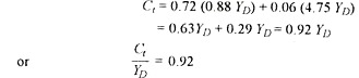
IMAGES

Relative Income Hypothesis
Relative Income Hypothesis (With Diagram)
Relative Income Hypothesis
Relative Income Hypothesis
RELATIVE INCOME HYPOTHESIS THEORY OF CONSUMPTION
Absolute, Relative and Permanent Income Hypothesis (With Diagram)

VIDEO

Economics terms
Relative Income Hypothesis/Theory || Short & Long Run || 4th Semester ||Urdu
Cool Graph on the Riemann Hypothesis💀😲
The Absolute Income hypothesis(Consumption)
Relative income hypothesis||Macroeconomics||MA economics
Absolute Income Hypothesis

COMMENTS

Relative Income Hypothesis (With Diagram)
Thus, under the relative income hypothesis, the basic function is the long-run function. The short-run consumption function is produced by cyclical movements in income. Suppose, in Figure 6.14, income has increased steadily to F 0 and consumption has increased to Co. Now suppose income falls to, say, Y 1. Instead of consumption falling to C 1 ...
Relative Income Hypothesis
Let us look at a relative income hypothesis example to understand the concept better. Alex earns $500 a month, and their consumption is $200 per month. Due to the recession, their income falls to $300 and their consumption to $170. But after the recession, the income steadily rises to $1000, and the consumption level rises to $400.
The relative income hypothesis
1. Introduction. Duesenberry (1949), in his seminal work, Income, Saving and the Theory of Consumer Behavior, introduces the relative income hypothesis in an attempt to rationalize the well established differences between cross-sectional and time-series properties of consumption data.On the one hand, a wealth of studies based on 1935-1936 and 1941-1942 cross-sectional budget surveys ...
PDF The relative income hypothesis
In order to illustrate our permanent income version of the relative income hypothesis it is convenient to define (actual) lifetime income as, where we have used (28) and (29). The saving and bequest rates out of (actual) lifetime income are the ratio of (26) and (29) to (30) respectively.
Relative income hypothesis
The relative income hypothesis was developed by James Duesenberry and states that an individual's attitude to consumption and saving is dictated more by his income in relation to others than by abstract standard of living.The percentage of income consumed by an individual depends on his percentile position within the income distribution.. It also hypothesizes that the present consumption is ...
PDF The Relation Between the Permanent Income and Relative Income Hypotheses
RELATION TO RELATIVE INCOME HYPOTHESIS 1. Relative Income Status Measured by Ratio -of Measured Income to Average Income Under these conditions, from (3.10) and (3.11), the regression of consumption on measured income is given by (6.1) c =k(1 — + Dividing both sides by y, we have (6.2) This is a linear relation between the consumption ratio ...
Relative Income Hypothesis
Abstract. The relative income hypothesis as expressed by its foremost exponent was an effort to reconcile conflicting evidence revealed by consumption functions fitted to long and short-period time series, and budget data; to bring social psychology into consumer theory; and to restore virtue to the act of saving (Duesenberry 1962).
Relative Income Hypothesis
However, relative income hypothesis proposes a slightly different utility function which can be stated as follows: According to this utility function, there is a positive relationship between utility and relative consumption. This means that utility will increase when consumption increases relative to the average consumption of the population.
The relative income hypothesis: A comparison of methods
The relative income (RI) hypothesis was proposed to explain savings behaviour in the US ( Duesenberry, 1949 ). The hypothesis, which states that individual utility depends both on own income and income relative to others, did not attract a lot of empirical attention until two separate later developments.
PDF The Relative Income and Relative Deprivation Hypotheses
hypothesis has become mainstream in economics. As aresult, tests of the relative income hypothesis havestarted to appear in high-ranking journals including the . Journal of Economic Literature, the . Economic Journal. and the . Journal of Public Economics, bringing to new life the original relative income hypothesis proposed by Duesemberry (1949).
Relative Income Hypothesis
Relative income hypothesis states that the satisfaction (or utility) an individual derives from a given consumption level depends on its relative magnitude in the society (e.g., relative to the average consumption) rather than its absolute level. It is based on a postulate that has long been acknowledged by psychologists and sociologists ...
The Relative Income and Relative Deprivation Hypotheses : A Review of
The paper provides a review of the empirical literature in economics that has attempted to test the relative income hypothesis as put forward by Duesemberry (1949) and the relative deprivation hypothesis as formalized by Runciman (1966). It is argued that these two hypotheses and the empirical models used to test them are essentially similar and make use of the same relative income concept.
9. Theories of Consumption
According to the relative income hypothesis, the fraction of a family's income that will be allocated to consumption will depend on its income level relative to the income level of the other families with which it classifies itself. The permanent income hypothesis puts forward the view that consumption is related to the permanent income.
Relative income hypothesis
Search for: 'relative income hypothesis' in Oxford Reference ». The theory that savings behaviour is affected by a person's relative position in the income distribution. Thus at a given level of real income, a person may be a relatively poor member of a rich community, or a relatively rich member of a poor community. The member of the richer ...
An Influence of Relative Income on the Marginal Propensity ...
2. Relative income hypothesis "Professor Duesenberry's study of the impact of budgetary and aggregative empirical consumption data on the received theory of consumer behavior is one of the most significant contributions of the postwar period to our understanding of economic behavior" written in his review by Arrow (1950, p. 906), his time respected neoclassical economist and later Nobel ...
Relative Income, Subjective Wellbeing and the Easterlin ...
A second explanation is the 'Relative Income Hypothesis' by which people derive utility from income in relation to other groups (Duesenberry 1949; Van Praag and Kapteyn ... Figures 4.3 and 4.4 graph RelGNDI for each of the country sub-sets for the period 1990-2009 showing considerable cross-country variation in RelGNDI for both country ...
The relative income hypothesis
Introduction. Duesenberry (1949), in his seminal work, Income, Saving and the Theory of Consumer Behavior, introduces the relative income hypothesis in an attempt to rationalize the well established differences between cross-sectional and time-series properties of consumption data. On the one hand, a wealth of studies based on 1935-1936 and ...
Absolute Income, Relative Income, and Happiness
The relative income hypothesis is also consistent with Easterlin's failure to find a strong association between income and happiness across countries: if absolute incomes were identically distributed around their means in all countries, the distribution of relative incomes would be identical across countries. ... regions on the graph. The ...
Mortality and distribution of income
Secondly, he says that the international association between inequalities in health and in income 3-1 supports the relative income hypothesis. In fact, this association is irrelevant for distinguishing between the relative and absolute income hypotheses. It would arise if health were positively related to income, in a linear or non-linear way.
What is the relative income hypothesis? Definition and meaning
The Relative Income Hypothesis says that we care more about how much we earn and consume in relation to how other people around us do than our absolute well-being or our own earnings and consumption in isolation or comparison to a moment in the past. According to relative income supposition, a typical person is happier if he or she got a $100 ...
Life Cycle Theories of Savings and Consumption
The life cycle hypothesis (LCH) is an alternative to earlier macroeconomic theories of savings and consumption, such as Keynes' absolute income hypothesis, Duesenberry's theory of relative income, or Fisher's theory of intertemporal choice (cf. Table 1).It assumes that savings and consumption depend on the average level of income over an extended period of human life, as opposed to the ...
The Life-Cycle Theory of Consumption (With Diagram)
Y-1e = the average annual labour income expected over the future (N - 1) years during which the individual plans to work . A t = the value of presently held assets . It can be seen from Equation (1) that according to the life cycle hypothesis, consumption depends not only on current income but also on expected future income and current asset holdings (i.e., current wealth).