sample hypothesis test

User Preferences

Content preview.

Arcu felis bibendum ut tristique et egestas quis:

• Ut enim ad minim veniam, quis nostrud exercitation ullamco laboris
• Duis aute irure dolor in reprehenderit in voluptate
• Excepteur sint occaecat cupidatat non proident

Keyboard Shortcuts

S.3 hypothesis testing.

In reviewing hypothesis tests, we start first with the general idea. Then, we keep returning to the basic procedures of hypothesis testing, each time adding a little more detail.

The general idea of hypothesis testing involves:

• Making an initial assumption.
• Collecting evidence (data).
• Based on the available evidence (data), deciding whether to reject or not reject the initial assumption.

Every hypothesis test — regardless of the population parameter involved — requires the above three steps.

Example S.3.1

Is normal body temperature really 98.6 degrees f section  .

Consider the population of many, many adults. A researcher hypothesized that the average adult body temperature is lower than the often-advertised 98.6 degrees F. That is, the researcher wants an answer to the question: "Is the average adult body temperature 98.6 degrees? Or is it lower?" To answer his research question, the researcher starts by assuming that the average adult body temperature was 98.6 degrees F.

Then, the researcher went out and tried to find evidence that refutes his initial assumption. In doing so, he selects a random sample of 130 adults. The average body temperature of the 130 sampled adults is 98.25 degrees.

Then, the researcher uses the data he collected to make a decision about his initial assumption. It is either likely or unlikely that the researcher would collect the evidence he did given his initial assumption that the average adult body temperature is 98.6 degrees:

• If it is likely , then the researcher does not reject his initial assumption that the average adult body temperature is 98.6 degrees. There is not enough evidence to do otherwise.
• either the researcher's initial assumption is correct and he experienced a very unusual event;
• or the researcher's initial assumption is incorrect.

In statistics, we generally don't make claims that require us to believe that a very unusual event happened. That is, in the practice of statistics, if the evidence (data) we collected is unlikely in light of the initial assumption, then we reject our initial assumption.

Example S.3.2

Criminal trial analogy section  .

One place where you can consistently see the general idea of hypothesis testing in action is in criminal trials held in the United States. Our criminal justice system assumes "the defendant is innocent until proven guilty." That is, our initial assumption is that the defendant is innocent.

In the practice of statistics, we make our initial assumption when we state our two competing hypotheses -- the null hypothesis ( H 0 ) and the alternative hypothesis ( H A ). Here, our hypotheses are:

• H 0 : Defendant is not guilty (innocent)
• H A : Defendant is guilty

In statistics, we always assume the null hypothesis is true . That is, the null hypothesis is always our initial assumption.

The prosecution team then collects evidence — such as finger prints, blood spots, hair samples, carpet fibers, shoe prints, ransom notes, and handwriting samples — with the hopes of finding "sufficient evidence" to make the assumption of innocence refutable.

In statistics, the data are the evidence.

The jury then makes a decision based on the available evidence:

• If the jury finds sufficient evidence — beyond a reasonable doubt — to make the assumption of innocence refutable, the jury rejects the null hypothesis and deems the defendant guilty. We behave as if the defendant is guilty.
• If there is insufficient evidence, then the jury does not reject the null hypothesis . We behave as if the defendant is innocent.

In statistics, we always make one of two decisions. We either "reject the null hypothesis" or we "fail to reject the null hypothesis."

Errors in Hypothesis Testing Section  

Did you notice the use of the phrase "behave as if" in the previous discussion? We "behave as if" the defendant is guilty; we do not "prove" that the defendant is guilty. And, we "behave as if" the defendant is innocent; we do not "prove" that the defendant is innocent.

This is a very important distinction! We make our decision based on evidence not on 100% guaranteed proof. Again:

• If we reject the null hypothesis, we do not prove that the alternative hypothesis is true.
• If we do not reject the null hypothesis, we do not prove that the null hypothesis is true.

We merely state that there is enough evidence to behave one way or the other. This is always true in statistics! Because of this, whatever the decision, there is always a chance that we made an error .

Let's review the two types of errors that can be made in criminal trials:

Table S.3.2 shows how this corresponds to the two types of errors in hypothesis testing.

Note that, in statistics, we call the two types of errors by two different  names -- one is called a "Type I error," and the other is called  a "Type II error." Here are the formal definitions of the two types of errors:

There is always a chance of making one of these errors. But, a good scientific study will minimize the chance of doing so!

Making the Decision Section  

Recall that it is either likely or unlikely that we would observe the evidence we did given our initial assumption. If it is likely , we do not reject the null hypothesis. If it is unlikely , then we reject the null hypothesis in favor of the alternative hypothesis. Effectively, then, making the decision reduces to determining "likely" or "unlikely."

In statistics, there are two ways to determine whether the evidence is likely or unlikely given the initial assumption:

• We could take the " critical value approach " (favored in many of the older textbooks).
• Or, we could take the " P -value approach " (what is used most often in research, journal articles, and statistical software).

In the next two sections, we review the procedures behind each of these two approaches. To make our review concrete, let's imagine that μ is the average grade point average of all American students who major in mathematics. We first review the critical value approach for conducting each of the following three hypothesis tests about the population mean $\mu$:

In Practice

• We would want to conduct the first hypothesis test if we were interested in concluding that the average grade point average of the group is more than 3.
• We would want to conduct the second hypothesis test if we were interested in concluding that the average grade point average of the group is less than 3.
• And, we would want to conduct the third hypothesis test if we were only interested in concluding that the average grade point average of the group differs from 3 (without caring whether it is more or less than 3).

Upon completing the review of the critical value approach, we review the P -value approach for conducting each of the above three hypothesis tests about the population mean \(\mu\). The procedures that we review here for both approaches easily extend to hypothesis tests about any other population parameter.

9.4 Full Hypothesis Test Examples

Tests on means, example 9.8.

Jeffrey, as an eight-year old, established a mean time of 16.43 seconds for swimming the 25-yard freestyle, with a standard deviation of 0.8 seconds . His dad, Frank, thought that Jeffrey could swim the 25-yard freestyle faster using goggles. Frank bought Jeffrey a new pair of expensive goggles and timed Jeffrey for 15 25-yard freestyle swims . For the 15 swims, Jeffrey's mean time was 16 seconds. Frank thought that the goggles helped Jeffrey to swim faster than the 16.43 seconds. Conduct a hypothesis test using a preset α = 0.05. Assume that the swim times for the 25-yard freestyle are normal.

Set up the Hypothesis Test:

Since the problem is about a mean, this is a test of a single population mean .

H 0 : μ = 16.43   H a : μ < 16.43

For Jeffrey to swim faster, his time will be less than 16.43 seconds. The "<" tells you this is left-tailed.

Determine the distribution needed:

Random variable: X ¯ X ¯ = the mean time to swim the 25-yard freestyle.

Distribution for the test: X ¯ X ¯ is normal (population standard deviation is known: σ = 0.8)

X ¯ ~ N ( μ , σ X n ) X ¯ ~ N ( μ , σ X n ) Therefore, X ¯ ~ N ( 16.43 , 0.8 15 ) X ¯ ~ N ( 16.43 , 0.8 15 )

μ = 16.43 comes from H 0 and not the data. σ = 0.8, and n = 15.

Calculate the p -value using the normal distribution for a mean:

p -value = P ( x ¯ x ¯ < 16) = 0.0187 where the sample mean in the problem is given as 16.

p -value = 0.0187 (This is called the actual level of significance .) The p -value is the area to the left of the sample mean is given as 16.

μ = 16.43 comes from H 0 . Our assumption is μ = 16.43.

Interpretation of the p -value: If H 0 is true , there is a 0.0187 probability (1.87%)that Jeffrey's mean time to swim the 25-yard freestyle is 16 seconds or less. Because a 1.87% chance is small, the mean time of 16 seconds or less is unlikely to have happened randomly. It is a rare event.

Compare α and the p -value:

α = 0.05 p -value = 0.0187 α > p -value

Make a decision: Since α > α > p -value, reject H 0 .

This indicates that you reject the null hypothesis that the mean time to swim the 25-yard freestyle is at least 16.43 seconds.

Conclusion: At the 5% significance level, there is sufficient evidence that Jeffrey's mean time to swim the 25-yard freestyle is less than 16.43 seconds. Thus, based on the sample data, we conclude that Jeffrey swims faster using the new goggles.

The Type I and Type II errors for this problem are as follows: The Type I error is to conclude that Jeffrey swims the 25-yard freestyle, on average, in less than 16.43 seconds when, in fact, he actually swims the 25-yard freestyle, on average, in at least 16.43 seconds. (Reject the null hypothesis when the null hypothesis is true.)

The Type II error is that there is not evidence to conclude that Jeffrey swims the 25-yard freestyle, on average, in less than 16.43 seconds when, in fact, he actually does swim the 25-yard free-style, on average, in less than 16.43 seconds. (Do not reject the null hypothesis when the null hypothesis is false.)

The mean throwing distance of a football for Marco, a high school quarterback, is 40 yards, with a standard deviation of two yards. The team coach tells Marco to adjust his grip to get more distance. The coach records the distances for 20 throws. For the 20 throws, Marco’s mean distance was 45 yards. The coach thought the different grip helped Marco throw farther than 40 yards. Conduct a hypothesis test using a preset α = 0.05. Assume the throw distances for footballs are normal.

First, determine what type of test this is, set up the hypothesis test, find the p -value, sketch the graph, and state your conclusion.

Example 9.9

Jasmine has just begun her new job on the sales force of a very competitive company. In a sample of 16 sales calls it was found that she closed the contract for an average value of 108 dollars with a standard deviation of 12 dollars. Test at 5% significance that the population mean is at least 100 dollars against the alternative that it is less than 100 dollars. Company policy requires that new members of the sales force must exceed an average of $100 per contract during the trial employment period. Can we conclude that Jasmine has met this requirement at the significance level of 95%?

• H 0 : µ ≤ 100 H a : µ > 100 The null and alternative hypothesis are for the parameter µ because the number of dollars of the contracts is a continuous random variable. Also, this is a one-tailed test because the company has only an interested if the number of dollars per contact is below a particular number not "too high" a number. This can be thought of as making a claim that the requirement is being met and thus the claim is in the alternative hypothesis.
• Test statistic: t c = x ¯ − µ 0 s n = 108 − 100 ( 12 16 ) = 2.67 t c = x ¯ − µ 0 s n = 108 − 100 ( 12 16 ) = 2.67
• Critical value: t a = 1.753 t a = 1.753 with n-1 degrees of freedom= 15

The test statistic is a Student's t because the sample size is below 30; therefore, we cannot use the normal distribution. Comparing the calculated value of the test statistic and the critical value of t t ( t a ) ( t a ) at a 5% significance level, we see that the calculated value is in the tail of the distribution. Thus, we conclude that 108 dollars per contract is significantly larger than the hypothesized value of 100 and thus we cannot accept the null hypothesis. There is evidence that supports Jasmine's performance meets company standards.

It is believed that a stock price for a particular company will grow at a rate of $5 per week with a standard deviation of $1. An investor believes the stock won’t grow as quickly. The changes in stock price is recorded for ten weeks and are as follows: $4, $3, $2, $3, $1, $7, $2, $1, $1, $2. Perform a hypothesis test using a 5% level of significance. State the null and alternative hypotheses, state your conclusion, and identify the Type I errors.

Example 9.10

A manufacturer of salad dressings uses machines to dispense liquid ingredients into bottles that move along a filling line. The machine that dispenses salad dressings is working properly when 8 ounces are dispensed. Suppose that the average amount dispensed in a particular sample of 35 bottles is 7.91 ounces with a variance of 0.03 ounces squared, s 2 s 2 . Is there evidence that the machine should be stopped and production wait for repairs? The lost production from a shutdown is potentially so great that management feels that the level of significance in the analysis should be 99%.

Again we will follow the steps in our analysis of this problem.

STEP 1 : Set the Null and Alternative Hypothesis. The random variable is the quantity of fluid placed in the bottles. This is a continuous random variable and the parameter we are interested in is the mean. Our hypothesis therefore is about the mean. In this case we are concerned that the machine is not filling properly. From what we are told it does not matter if the machine is over-filling or under-filling, both seem to be an equally bad error. This tells us that this is a two-tailed test: if the machine is malfunctioning it will be shutdown regardless if it is from over-filling or under-filling. The null and alternative hypotheses are thus:

STEP 2 : Decide the level of significance and draw the graph showing the critical value.

This problem has already set the level of significance at 99%. The decision seems an appropriate one and shows the thought process when setting the significance level. Management wants to be very certain, as certain as probability will allow, that they are not shutting down a machine that is not in need of repair. To draw the distribution and the critical value, we need to know which distribution to use. Because this is a continuous random variable and we are interested in the mean, and the sample size is greater than 30, the appropriate distribution is the normal distribution and the relevant critical value is 2.575 from the normal table or the t-table at 0.005 column and infinite degrees of freedom. We draw the graph and mark these points.

STEP 3 : Calculate sample parameters and the test statistic. The sample parameters are provided, the sample mean is 7.91 and the sample variance is .03 and the sample size is 35. We need to note that the sample variance was provided not the sample standard deviation, which is what we need for the formula. Remembering that the standard deviation is simply the square root of the variance, we therefore know the sample standard deviation, s, is 0.173. With this information we calculate the test statistic as -3.07, and mark it on the graph.

STEP 4 : Compare test statistic and the critical values Now we compare the test statistic and the critical value by placing the test statistic on the graph. We see that the test statistic is in the tail, decidedly greater than the critical value of 2.575. We note that even the very small difference between the hypothesized value and the sample value is still a large number of standard deviations. The sample mean is only 0.08 ounces different from the required level of 8 ounces, but it is 3 plus standard deviations away and thus we cannot accept the null hypothesis.

STEP 5 : Reach a Conclusion

Three standard deviations of a test statistic will guarantee that the test will fail. The probability that anything is within three standard deviations is almost zero. Actually it is 0.0026 on the normal distribution, which is certainly almost zero in a practical sense. Our formal conclusion would be “ At a 99% level of significance we cannot accept the hypothesis that the sample mean came from a distribution with a mean of 8 ounces” Or less formally, and getting to the point, “At a 99% level of significance we conclude that the machine is under filling the bottles and is in need of repair”.

Try It 9.10

A company records the mean time of employees working in a day. The mean comes out to be 475 minutes, with a standard deviation of 45 minutes. A manager recorded times of 20 employees. The times of working were (frequencies are in parentheses) 460(3); 465(2); 470(3); 475(1); 480(6); 485(3); 490(2).

Conduct a hypothesis test using a 2.5% level of significance to determine if the mean time is more than 475 .

Hypothesis Test for Proportions

Just as there were confidence intervals for proportions, or more formally, the population parameter p of the binomial distribution, there is the ability to test hypotheses concerning p .

The population parameter for the binomial is p . The estimated value (point estimate) for p is p′ where p′ = x/n , x is the number of successes in the sample and n is the sample size.

When you perform a hypothesis test of a population proportion p , you take a simple random sample from the population. The conditions for a binomial distribution must be met, which are: there are a certain number n of independent trials meaning random sampling, the outcomes of any trial are binary, success or failure, and each trial has the same probability of a success p . The shape of the binomial distribution needs to be similar to the shape of the normal distribution. To ensure this, the quantities np′ and nq′ must both be greater than five ( np′ > 5 and nq′ > 5). In this case the binomial distribution of a sample (estimated) proportion can be approximated by the normal distribution with μ = np μ = np and σ = npq σ = npq . Remember that q = 1 – p q = 1 – p . There is no distribution that can correct for this small sample bias and thus if these conditions are not met we simply cannot test the hypothesis with the data available at that time. We met this condition when we first were estimating confidence intervals for p .

Again, we begin with the standardizing formula modified because this is the distribution of a binomial.

Substituting p 0 p 0 , the hypothesized value of p , we have:

This is the test statistic for testing hypothesized values of p , where the null and alternative hypotheses take one of the following forms:

The decision rule stated above applies here also: if the calculated value of Z c shows that the sample proportion is "too many" standard deviations from the hypothesized proportion, the null hypothesis cannot be accepted. The decision as to what is "too many" is pre-determined by the analyst depending on the level of significance required in the test.

Example 9.11

The mortgage department of a large bank is interested in the nature of loans of first-time borrowers. This information will be used to tailor their marketing strategy. They believe that 50% of first-time borrowers take out smaller loans than other borrowers. They perform a hypothesis test to determine if the percentage is the same or different from 50% . They sample 100 first-time borrowers and find 53 of these loans are smaller that the other borrowers. For the hypothesis test, they choose a 5% level of significance.

STEP 1 : Set the null and alternative hypothesis.

H 0 : p = 0.50   H a : p ≠ 0.50

The words "is the same or different from" tell you this is a two-tailed test. The Type I and Type II errors are as follows: The Type I error is to conclude that the proportion of borrowers is different from 50% when, in fact, the proportion is actually 50%. (Reject the null hypothesis when the null hypothesis is true). The Type II error is there is not enough evidence to conclude that the proportion of first time borrowers differs from 50% when, in fact, the proportion does differ from 50%. (You fail to reject the null hypothesis when the null hypothesis is false.)

STEP 2 : Decide the level of significance and draw the graph showing the critical value

The level of significance has been set by the problem at the 5% level. Because this is two-tailed test one-half of the alpha value will be in the upper tail and one-half in the lower tail as shown on the graph. The critical value for the normal distribution at the 95% level of confidence is 1.96. This can easily be found on the student’s t-table at the very bottom at infinite degrees of freedom remembering that at infinity the t-distribution is the normal distribution. Of course the value can also be found on the normal table but you have go looking for one-half of 95 (0.475) inside the body of the table and then read out to the sides and top for the number of standard deviations.

STEP 3 : Calculate the sample parameters and critical value of the test statistic.

The test statistic is a normal distribution, Z, for testing proportions and is:

For this case, the sample of 100 found 53 of these loans were smaller than those of other borrowers. The sample proportion, p′ = 53/100= 0.53 The test question, therefore, is : “Is 0.53 significantly different from .50?” Putting these values into the formula for the test statistic we find that 0.53 is only 0.60 standard deviations away from .50. This is barely off of the mean of the standard normal distribution of zero. There is virtually no difference from the sample proportion and the hypothesized proportion in terms of standard deviations.

STEP 4 : Compare the test statistic and the critical value.

The calculated value is well within the critical values of ± 1.96 standard deviations and thus we cannot reject the null hypothesis. To reject the null hypothesis we need significant evident of difference between the hypothesized value and the sample value. In this case the sample value is very nearly the same as the hypothesized value measured in terms of standard deviations.

STEP 5 : Reach a conclusion

The formal conclusion would be “At a 5% level of significance we cannot reject the null hypothesis that 50% of first-time borrowers take out smaller loans than other borrowers.” Notice the length to which the conclusion goes to include all of the conditions that are attached to the conclusion. Statisticians, for all the criticism they receive, are careful to be very specific even when this seems trivial. Statisticians cannot say more than they know, and the data constrain the conclusion to be within the metes and bounds of the data.

Try It 9.11

A teacher believes that 85% of students in the class will want to go on a field trip to the local zoo. The teacher performs a hypothesis test to determine if the percentage is the same or different from 85%. The teacher samples 50 students and 39 reply that they would want to go to the zoo. For the hypothesis test, use a 1% level of significance.

Example 9.12

Suppose a consumer group suspects that the proportion of households that have three or more cell phones is 30%. A cell phone company has reason to believe that the proportion is not 30%. Before they start a big advertising campaign, they conduct a hypothesis test. Their marketing people survey 150 households with the result that 43 of the households have three or more cell phones.

Here is an abbreviate version of the system to solve hypothesis tests applied to a test on a proportions.

Try It 9.12

Marketers believe that 92% of adults in the United States own a cell phone. A cell phone manufacturer believes that number is actually lower. 200 American adults are surveyed, of which, 174 report having cell phones. Use a 5% level of significance. State the null and alternative hypothesis, find the p -value, state your conclusion, and identify the Type I and Type II errors.

Example 9.13

The National Institute of Standards and Technology provides exact data on conductivity properties of materials. Following are conductivity measurements for 11 randomly selected pieces of a particular type of glass.

1.11; 1.07; 1.11; 1.07; 1.12; 1.08; .98; .98; 1.02; .95; .95 Is there convincing evidence that the average conductivity of this type of glass is greater than one? Use a significance level of 0.05.

Let’s follow a four-step process to answer this statistical question.

• H 0 : μ ≤ 1
• H a : μ > 1
• Plan : We are testing a sample mean without a known population standard deviation with less than 30 observations. Therefore, we need to use a Student's-t distribution. Assume the underlying population is normal.
• Do the calculations and draw the graph .
• State the Conclusions : We cannot accept the null hypothesis. It is reasonable to state that the data supports the claim that the average conductivity level is greater than one.

Try It 9.13

The boiling point of a specific liquid is measured for 15 samples, and the boiling points are obtained as follows:

205; 206; 206; 202; 199; 194; 197; 198; 198; 201; 201; 202; 207; 211; 205

Is there convincing evidence that the average boiling point is greater than 200? Use a significance level of 0.1. Assume the population is normal.

Example 9.14

In a study of 420,019 cell phone users, 172 of the subjects developed brain cancer. Test the claim that cell phone users developed brain cancer at a greater rate than that for non-cell phone users (the rate of brain cancer for non-cell phone users is 0.0340%). Since this is a critical issue, use a 0.005 significance level. Explain why the significance level should be so low in terms of a Type I error.

• H 0 : p ≤ 0.00034
• H a : p > 0.00034

If we commit a Type I error, we are essentially accepting a false claim. Since the claim describes cancer-causing environments, we want to minimize the chances of incorrectly identifying causes of cancer.

• We will be testing a sample proportion with x = 172 and n = 420,019. The sample is sufficiently large because we have np' = 420,019(0.00034) = 142.8, nq' = 420,019(0.99966) = 419,876.2, two independent outcomes, and a fixed probability of success p' = 0.00034. Thus we will be able to generalize our results to the population.

Try It 9.14

In a study of 390,000 moisturizer users, 138 of the subjects developed skin diseases. Test the claim that moisturizer users developed skin diseases at a greater rate than that for non-moisturizer users (the rate of skin diseases for non-moisturizer users is 0.041%). Since this is a critical issue, use a 0.005 significance level. Explain why the significance level should be so low in terms of a Type I error.

This book may not be used in the training of large language models or otherwise be ingested into large language models or generative AI offerings without OpenStax's permission.

Want to cite, share, or modify this book? This book uses the Creative Commons Attribution License and you must attribute OpenStax.

Access for free at https://openstax.org/books/introductory-business-statistics-2e/pages/1-introduction

• Authors: Alexander Holmes, Barbara Illowsky, Susan Dean
• Publisher/website: OpenStax
• Book title: Introductory Business Statistics 2e
• Publication date: Dec 13, 2023
• Location: Houston, Texas
• Book URL: https://openstax.org/books/introductory-business-statistics-2e/pages/1-introduction
• Section URL: https://openstax.org/books/introductory-business-statistics-2e/pages/9-4-full-hypothesis-test-examples

© Dec 6, 2023 OpenStax. Textbook content produced by OpenStax is licensed under a Creative Commons Attribution License . The OpenStax name, OpenStax logo, OpenStax book covers, OpenStax CNX name, and OpenStax CNX logo are not subject to the Creative Commons license and may not be reproduced without the prior and express written consent of Rice University.

Hypothesis Testing

Hypothesis testing is a tool for making statistical inferences about the population data. It is an analysis tool that tests assumptions and determines how likely something is within a given standard of accuracy. Hypothesis testing provides a way to verify whether the results of an experiment are valid.

A null hypothesis and an alternative hypothesis are set up before performing the hypothesis testing. This helps to arrive at a conclusion regarding the sample obtained from the population. In this article, we will learn more about hypothesis testing, its types, steps to perform the testing, and associated examples.

What is Hypothesis Testing in Statistics?

Hypothesis testing uses sample data from the population to draw useful conclusions regarding the population probability distribution . It tests an assumption made about the data using different types of hypothesis testing methodologies. The hypothesis testing results in either rejecting or not rejecting the null hypothesis.

Hypothesis Testing Definition

Hypothesis testing can be defined as a statistical tool that is used to identify if the results of an experiment are meaningful or not. It involves setting up a null hypothesis and an alternative hypothesis. These two hypotheses will always be mutually exclusive. This means that if the null hypothesis is true then the alternative hypothesis is false and vice versa. An example of hypothesis testing is setting up a test to check if a new medicine works on a disease in a more efficient manner.

Null Hypothesis

The null hypothesis is a concise mathematical statement that is used to indicate that there is no difference between two possibilities. In other words, there is no difference between certain characteristics of data. This hypothesis assumes that the outcomes of an experiment are based on chance alone. It is denoted as \(H_{0}\). Hypothesis testing is used to conclude if the null hypothesis can be rejected or not. Suppose an experiment is conducted to check if girls are shorter than boys at the age of 5. The null hypothesis will say that they are the same height.

Alternative Hypothesis

The alternative hypothesis is an alternative to the null hypothesis. It is used to show that the observations of an experiment are due to some real effect. It indicates that there is a statistical significance between two possible outcomes and can be denoted as \(H_{1}\) or \(H_{a}\). For the above-mentioned example, the alternative hypothesis would be that girls are shorter than boys at the age of 5.

Hypothesis Testing P Value

In hypothesis testing, the p value is used to indicate whether the results obtained after conducting a test are statistically significant or not. It also indicates the probability of making an error in rejecting or not rejecting the null hypothesis.This value is always a number between 0 and 1. The p value is compared to an alpha level, \(\alpha\) or significance level. The alpha level can be defined as the acceptable risk of incorrectly rejecting the null hypothesis. The alpha level is usually chosen between 1% to 5%.

Hypothesis Testing Critical region

All sets of values that lead to rejecting the null hypothesis lie in the critical region. Furthermore, the value that separates the critical region from the non-critical region is known as the critical value.

Hypothesis Testing Formula

Depending upon the type of data available and the size, different types of hypothesis testing are used to determine whether the null hypothesis can be rejected or not. The hypothesis testing formula for some important test statistics are given below:

• z = \(\frac{\overline{x}-\mu}{\frac{\sigma}{\sqrt{n}}}\). \(\overline{x}\) is the sample mean, \(\mu\) is the population mean, \(\sigma\) is the population standard deviation and n is the size of the sample.
• t = \(\frac{\overline{x}-\mu}{\frac{s}{\sqrt{n}}}\). s is the sample standard deviation.
• \(\chi ^{2} = \sum \frac{(O_{i}-E_{i})^{2}}{E_{i}}\). \(O_{i}\) is the observed value and \(E_{i}\) is the expected value.

We will learn more about these test statistics in the upcoming section.

Types of Hypothesis Testing

Selecting the correct test for performing hypothesis testing can be confusing. These tests are used to determine a test statistic on the basis of which the null hypothesis can either be rejected or not rejected. Some of the important tests used for hypothesis testing are given below.

Hypothesis Testing Z Test

A z test is a way of hypothesis testing that is used for a large sample size (n ≥ 30). It is used to determine whether there is a difference between the population mean and the sample mean when the population standard deviation is known. It can also be used to compare the mean of two samples. It is used to compute the z test statistic. The formulas are given as follows:

• One sample: z = \(\frac{\overline{x}-\mu}{\frac{\sigma}{\sqrt{n}}}\).
• Two samples: z = \(\frac{(\overline{x_{1}}-\overline{x_{2}})-(\mu_{1}-\mu_{2})}{\sqrt{\frac{\sigma_{1}^{2}}{n_{1}}+\frac{\sigma_{2}^{2}}{n_{2}}}}\).

Hypothesis Testing t Test

The t test is another method of hypothesis testing that is used for a small sample size (n < 30). It is also used to compare the sample mean and population mean. However, the population standard deviation is not known. Instead, the sample standard deviation is known. The mean of two samples can also be compared using the t test.

• One sample: t = \(\frac{\overline{x}-\mu}{\frac{s}{\sqrt{n}}}\).
• Two samples: t = \(\frac{(\overline{x_{1}}-\overline{x_{2}})-(\mu_{1}-\mu_{2})}{\sqrt{\frac{s_{1}^{2}}{n_{1}}+\frac{s_{2}^{2}}{n_{2}}}}\).

Hypothesis Testing Chi Square

The Chi square test is a hypothesis testing method that is used to check whether the variables in a population are independent or not. It is used when the test statistic is chi-squared distributed.

One Tailed Hypothesis Testing

One tailed hypothesis testing is done when the rejection region is only in one direction. It can also be known as directional hypothesis testing because the effects can be tested in one direction only. This type of testing is further classified into the right tailed test and left tailed test.

Right Tailed Hypothesis Testing

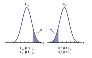
The right tail test is also known as the upper tail test. This test is used to check whether the population parameter is greater than some value. The null and alternative hypotheses for this test are given as follows:

\(H_{0}\): The population parameter is ≤ some value

\(H_{1}\): The population parameter is > some value.

If the test statistic has a greater value than the critical value then the null hypothesis is rejected

Left Tailed Hypothesis Testing

The left tail test is also known as the lower tail test. It is used to check whether the population parameter is less than some value. The hypotheses for this hypothesis testing can be written as follows:

\(H_{0}\): The population parameter is ≥ some value

\(H_{1}\): The population parameter is < some value.

The null hypothesis is rejected if the test statistic has a value lesser than the critical value.

Two Tailed Hypothesis Testing

In this hypothesis testing method, the critical region lies on both sides of the sampling distribution. It is also known as a non - directional hypothesis testing method. The two-tailed test is used when it needs to be determined if the population parameter is assumed to be different than some value. The hypotheses can be set up as follows:

\(H_{0}\): the population parameter = some value

\(H_{1}\): the population parameter ≠ some value

The null hypothesis is rejected if the test statistic has a value that is not equal to the critical value.

Hypothesis Testing Steps

Hypothesis testing can be easily performed in five simple steps. The most important step is to correctly set up the hypotheses and identify the right method for hypothesis testing. The basic steps to perform hypothesis testing are as follows:

• Step 1: Set up the null hypothesis by correctly identifying whether it is the left-tailed, right-tailed, or two-tailed hypothesis testing.
• Step 2: Set up the alternative hypothesis.
• Step 3: Choose the correct significance level, \(\alpha\), and find the critical value.
• Step 4: Calculate the correct test statistic (z, t or \(\chi\)) and p-value.
• Step 5: Compare the test statistic with the critical value or compare the p-value with \(\alpha\) to arrive at a conclusion. In other words, decide if the null hypothesis is to be rejected or not.

Hypothesis Testing Example

The best way to solve a problem on hypothesis testing is by applying the 5 steps mentioned in the previous section. Suppose a researcher claims that the mean average weight of men is greater than 100kgs with a standard deviation of 15kgs. 30 men are chosen with an average weight of 112.5 Kgs. Using hypothesis testing, check if there is enough evidence to support the researcher's claim. The confidence interval is given as 95%.

Step 1: This is an example of a right-tailed test. Set up the null hypothesis as \(H_{0}\): \(\mu\) = 100.

Step 2: The alternative hypothesis is given by \(H_{1}\): \(\mu\) > 100.

Step 3: As this is a one-tailed test, \(\alpha\) = 100% - 95% = 5%. This can be used to determine the critical value.

1 - \(\alpha\) = 1 - 0.05 = 0.95

0.95 gives the required area under the curve. Now using a normal distribution table, the area 0.95 is at z = 1.645. A similar process can be followed for a t-test. The only additional requirement is to calculate the degrees of freedom given by n - 1.

Step 4: Calculate the z test statistic. This is because the sample size is 30. Furthermore, the sample and population means are known along with the standard deviation.

z = \(\frac{\overline{x}-\mu}{\frac{\sigma}{\sqrt{n}}}\).

\(\mu\) = 100, \(\overline{x}\) = 112.5, n = 30, \(\sigma\) = 15

z = \(\frac{112.5-100}{\frac{15}{\sqrt{30}}}\) = 4.56

Step 5: Conclusion. As 4.56 > 1.645 thus, the null hypothesis can be rejected.

Hypothesis Testing and Confidence Intervals

Confidence intervals form an important part of hypothesis testing. This is because the alpha level can be determined from a given confidence interval. Suppose a confidence interval is given as 95%. Subtract the confidence interval from 100%. This gives 100 - 95 = 5% or 0.05. This is the alpha value of a one-tailed hypothesis testing. To obtain the alpha value for a two-tailed hypothesis testing, divide this value by 2. This gives 0.05 / 2 = 0.025.

Related Articles:

• Probability and Statistics
• Data Handling

Important Notes on Hypothesis Testing

• Hypothesis testing is a technique that is used to verify whether the results of an experiment are statistically significant.
• It involves the setting up of a null hypothesis and an alternate hypothesis.
• There are three types of tests that can be conducted under hypothesis testing - z test, t test, and chi square test.
• Hypothesis testing can be classified as right tail, left tail, and two tail tests.

Examples on Hypothesis Testing

• Example 1: The average weight of a dumbbell in a gym is 90lbs. However, a physical trainer believes that the average weight might be higher. A random sample of 5 dumbbells with an average weight of 110lbs and a standard deviation of 18lbs. Using hypothesis testing check if the physical trainer's claim can be supported for a 95% confidence level. Solution: As the sample size is lesser than 30, the t-test is used. \(H_{0}\): \(\mu\) = 90, \(H_{1}\): \(\mu\) > 90 \(\overline{x}\) = 110, \(\mu\) = 90, n = 5, s = 18. \(\alpha\) = 0.05 Using the t-distribution table, the critical value is 2.132 t = \(\frac{\overline{x}-\mu}{\frac{s}{\sqrt{n}}}\) t = 2.484 As 2.484 > 2.132, the null hypothesis is rejected. Answer: The average weight of the dumbbells may be greater than 90lbs
• Example 2: The average score on a test is 80 with a standard deviation of 10. With a new teaching curriculum introduced it is believed that this score will change. On random testing, the score of 38 students, the mean was found to be 88. With a 0.05 significance level, is there any evidence to support this claim? Solution: This is an example of two-tail hypothesis testing. The z test will be used. \(H_{0}\): \(\mu\) = 80, \(H_{1}\): \(\mu\) ≠ 80 \(\overline{x}\) = 88, \(\mu\) = 80, n = 36, \(\sigma\) = 10. \(\alpha\) = 0.05 / 2 = 0.025 The critical value using the normal distribution table is 1.96 z = \(\frac{\overline{x}-\mu}{\frac{\sigma}{\sqrt{n}}}\) z = \(\frac{88-80}{\frac{10}{\sqrt{36}}}\) = 4.8 As 4.8 > 1.96, the null hypothesis is rejected. Answer: There is a difference in the scores after the new curriculum was introduced.
• Example 3: The average score of a class is 90. However, a teacher believes that the average score might be lower. The scores of 6 students were randomly measured. The mean was 82 with a standard deviation of 18. With a 0.05 significance level use hypothesis testing to check if this claim is true. Solution: The t test will be used. \(H_{0}\): \(\mu\) = 90, \(H_{1}\): \(\mu\) < 90 \(\overline{x}\) = 110, \(\mu\) = 90, n = 6, s = 18 The critical value from the t table is -2.015 t = \(\frac{\overline{x}-\mu}{\frac{s}{\sqrt{n}}}\) t = \(\frac{82-90}{\frac{18}{\sqrt{6}}}\) t = -1.088 As -1.088 > -2.015, we fail to reject the null hypothesis. Answer: There is not enough evidence to support the claim.

go to slide go to slide go to slide

Book a Free Trial Class

FAQs on Hypothesis Testing

What is hypothesis testing.

Hypothesis testing in statistics is a tool that is used to make inferences about the population data. It is also used to check if the results of an experiment are valid.

What is the z Test in Hypothesis Testing?

The z test in hypothesis testing is used to find the z test statistic for normally distributed data . The z test is used when the standard deviation of the population is known and the sample size is greater than or equal to 30.

What is the t Test in Hypothesis Testing?

The t test in hypothesis testing is used when the data follows a student t distribution . It is used when the sample size is less than 30 and standard deviation of the population is not known.

What is the formula for z test in Hypothesis Testing?

The formula for a one sample z test in hypothesis testing is z = \(\frac{\overline{x}-\mu}{\frac{\sigma}{\sqrt{n}}}\) and for two samples is z = \(\frac{(\overline{x_{1}}-\overline{x_{2}})-(\mu_{1}-\mu_{2})}{\sqrt{\frac{\sigma_{1}^{2}}{n_{1}}+\frac{\sigma_{2}^{2}}{n_{2}}}}\).

What is the p Value in Hypothesis Testing?

The p value helps to determine if the test results are statistically significant or not. In hypothesis testing, the null hypothesis can either be rejected or not rejected based on the comparison between the p value and the alpha level.

What is One Tail Hypothesis Testing?

When the rejection region is only on one side of the distribution curve then it is known as one tail hypothesis testing. The right tail test and the left tail test are two types of directional hypothesis testing.

What is the Alpha Level in Two Tail Hypothesis Testing?

To get the alpha level in a two tail hypothesis testing divide \(\alpha\) by 2. This is done as there are two rejection regions in the curve.

Want to create or adapt books like this? Learn more about how Pressbooks supports open publishing practices.

11 Hypothesis Testing with One Sample

Student learning outcomes.

By the end of this chapter, the student should be able to:

• Be able to identify and develop the null and alternative hypothesis
• Identify the consequences of Type I and Type II error.
• Be able to perform an one-tailed and two-tailed hypothesis test using the critical value method
• Be able to perform a hypothesis test using the p-value method
• Be able to write conclusions based on hypothesis tests.

Introduction

Now we are down to the bread and butter work of the statistician: developing and testing hypotheses. It is important to   put this material in a broader context so that the method by which a hypothesis is formed is understood completely. Using textbook examples often clouds the real source of statistical hypotheses.

Statistical testing is part of a much larger process known as the scientific method. This method was developed more than two centuries ago as the accepted way that new knowledge could be created. Until then, and unfortunately even today, among some, “knowledge” could be created simply by some authority saying something was so, ipso dicta . Superstition and conspiracy theories were (are?) accepted uncritically.

The scientific method, briefly, states that only by following a careful and specific process can some assertion be included in the accepted body of knowledge. This process begins with a set of assumptions upon which a theory, sometimes called a model, is built. This theory, if it has any validity, will lead to predictions; what we call hypotheses.

As an example, in Microeconomics the theory of consumer choice begins with certain assumption concerning human behavior. From these assumptions a theory of how consumers make choices using indifference curves and the budget line. This theory gave rise to a very important prediction, namely, that there was an inverse relationship between price and quantity demanded. This relationship was known as the demand curve. The negative slope of the demand curve is really just a prediction, or a hypothesis, that can be tested with statistical tools.

Unless hundreds and hundreds of statistical tests of this hypothesis had not confirmed this relationship, the so-called Law of Demand would have been discarded years ago. This is the role of statistics, to test the hypotheses of various theories to determine if they should be admitted into the accepted body of knowledge; how we understand our world. Once admitted, however, they may be later discarded if new theories come along that make better predictions.

Not long ago two scientists claimed that they could get more energy out of a process than was put in. This caused a tremendous stir for obvious reasons. They were on the cover of Time and were offered extravagant sums to bring their research work to private industry and any number of universities. It was not long until their work was subjected to the rigorous tests of the scientific method and found to be a failure. No other lab could replicate their findings. Consequently they have sunk into obscurity and their theory discarded. It may surface again when someone can pass the tests of the hypotheses required by the scientific method, but until then it is just a curiosity. Many pure frauds have been attempted over time, but most have been found out by applying the process of the scientific method.

This discussion is meant to show just where in this process statistics falls. Statistics and statisticians are not necessarily in the business of developing theories, but in the business of testing others’ theories. Hypotheses come from these theories based upon an explicit set of assumptions and sound logic. The hypothesis comes first, before any data are gathered. Data do not create hypotheses; they are used to test them. If we bear this in mind as we study this section the process of forming and testing hypotheses will make more sense.

One job of a statistician is to make statistical inferences about populations based on samples taken from the population. Confidence intervals are one way to estimate a population parameter. Another way to make a statistical inference is to make a decision about the value of a specific parameter. For instance, a car dealer advertises that its new small truck gets 35 miles per gallon, on average. A tutoring service claims that its method of tutoring helps 90% of its students get an A or a B. A company says that women managers in their company earn an average of $60,000 per year.

A statistician will make a decision about these claims. This process is called ” hypothesis testing .” A hypothesis test involves collecting data from a sample and evaluating the data. Then, the statistician makes a decision as to whether or not there is sufficient evidence, based upon analyses of the data, to reject the null hypothesis.

In this chapter, you will conduct hypothesis tests on single means and single proportions. You will also learn about the errors associated with these tests.

Null and Alternative Hypotheses

The actual test begins by considering two hypotheses . They are called the null hypothesis and the alternative hypothesis . These hypotheses contain opposing viewpoints.

Since the null and alternative hypotheses are contradictory, you must examine evidence to decide if you have enough evidence to reject the null hypothesis or not. The evidence is in the form of sample data.

Table 1 presents the various hypotheses in the relevant pairs. For example, if the null hypothesis is equal to some value, the alternative has to be not equal to that value.

NOTE                                                                             

We want to test whether the mean GPA of students in American colleges is different from 2.0 (out of 4.0). The null and alternative hypotheses are:

We want to test if college students take less than five years to graduate from college, on the average. The null and alternative hypotheses are:

Outcomes and the Type I and Type II Errors

The four possible outcomes in the table are:

Each of the errors occurs with a particular probability. The Greek letters α and β represent the probabilities.

By way of example, the American judicial system begins with the concept that a defendant is “presumed innocent”. This is the status quo and is the null hypothesis. The judge will tell the jury that they can not find the defendant guilty unless the evidence indicates guilt beyond a “reasonable doubt” which is usually defined in criminal cases as 95% certainty of guilt. If the jury cannot accept the null, innocent, then action will be taken, jail time. The burden of proof always lies with the alternative hypothesis. (In civil cases, the jury needs only to be more than 50% certain of wrongdoing to find culpability, called “a preponderance of the evidence”).

The example above was for a test of a mean, but the same logic applies to tests of hypotheses for all statistical parameters one may wish to test.

The following are examples of Type I and Type II errors.

Type I error : Frank thinks that his rock climbing equipment may not be safe when, in fact, it really is safe.

Type II error : Frank thinks that his rock climbing equipment may be safe when, in fact, it is not safe.

Notice that, in this case, the error with the greater consequence is the Type II error. (If Frank thinks his rock climbing equipment is safe, he will go ahead and use it.)

This is a situation described as “accepting a false null”.

Type I error : The emergency crew thinks that the victim is dead when, in fact, the victim is alive. Type II error : The emergency crew does not know if the victim is alive when, in fact, the victim is dead.

The error with the greater consequence is the Type I error. (If the emergency crew thinks the victim is dead, they will not treat him.)

Distribution Needed for Hypothesis Testing

Particular distributions are associated with hypothesis testing.We will perform hypotheses tests of a population mean using a normal distribution or a Student’s t -distribution. (Remember, use a Student’s t -distribution when the population standard deviation is unknown and the sample size is small, where small is considered to be less than 30 observations.) We perform tests of a population proportion using a normal distribution when we can assume that the distribution is normally distributed. We consider this to be true if the sample proportion, p ‘ , times the sample size is greater than 5 and 1- p ‘ times the sample size is also greater then 5. This is the same rule of thumb we used when developing the formula for the confidence interval for a population proportion.

Hypothesis Test for the Mean

Going back to the standardizing formula we can derive the test statistic for testing hypotheses concerning means.

This gives us the decision rule for testing a hypothesis for a two-tailed test:

P-Value Approach

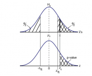
Both decision rules will result in the same decision and it is a matter of preference which one is used.

One and Two-tailed Tests

The claim would be in the alternative hypothesis. The burden of proof in hypothesis testing is carried in the alternative. This is because failing to reject the null, the status quo, must be accomplished with 90 or 95 percent significance that it cannot be maintained. Said another way, we want to have only a 5 or 10 percent probability of making a Type I error, rejecting a good null; overthrowing the status quo.

Figure 5 shows the two possible cases and the form of the null and alternative hypothesis that give rise to them.

Effects of Sample Size on Test Statistic

Table 3 summarizes test statistics for varying sample sizes and population standard deviation known and unknown.

A Systematic Approach for Testing A Hypothesis

A systematic approach to hypothesis testing follows the following steps and in this order. This template will work for all hypotheses that you will ever test.

• Set up the null and alternative hypothesis. This is typically the hardest part of the process. Here the question being asked is reviewed. What parameter is being tested, a mean, a proportion, differences in means, etc. Is this a one-tailed test or two-tailed test? Remember, if someone is making a claim it will always be a one-tailed test.
• Decide the level of significance required for this particular case and determine the critical value. These can be found in the appropriate statistical table. The levels of confidence typical for the social sciences are 90, 95 and 99. However, the level of significance is a policy decision and should be based upon the risk of making a Type I error, rejecting a good null. Consider the consequences of making a Type I error.
• Take a sample(s) and calculate the relevant parameters: sample mean, standard deviation, or proportion. Using the formula for the test statistic from above in step 2, now calculate the test statistic for this particular case using the parameters you have just calculated.
• Compare the calculated test statistic and the critical value. Marking these on the graph will give a good visual picture of the situation. There are now only two situations:

a.     The test statistic is in the tail: Cannot Accept the null, the probability that this sample mean (proportion) came from the hypothesized distribution is too small to believe that it is the real home of these sample data.

b.   The test statistic is not in the tail: Cannot Reject the null, the sample data are compatible with the hypothesized population parameter.

• Reach a conclusion. It is best to articulate the conclusion two different ways. First a formal statistical conclusion such as “With a 95 % level of significance we cannot accept the null hypotheses that the population mean is equal to XX (units of measurement)”. The second statement of the conclusion is less formal and states the action, or lack of action, required. If the formal conclusion was that above, then the informal one might be, “The machine is broken and we need to shut it down and call for repairs”.

All hypotheses tested will go through this same process. The only changes are the relevant formulas and those are determined by the hypothesis required to answer the original question.

Full Hypothesis Test Examples

Tests on means.

Jeffrey, as an eight-year old, established a mean time of 16.43 seconds for swimming the 25-yard freestyle, with a standard deviation of 0.8 seconds . His dad, Frank, thought that Jeffrey could swim the 25-yard freestyle faster using goggles. Frank bought Jeffrey a new pair of expensive goggles and timed Jeffrey for 15 25-yard freestyle swims . For the 15 swims, Jeffrey’s mean time was 16 seconds. Frank thought that the goggles helped Jeffrey to swim faster than the 16.43 seconds. Conduct a hypothesis test using a preset α = 0.05.

Solution – Example 6

Set up the Hypothesis Test:

Since the problem is about a mean, this is a test of a single population mean . Set the null and alternative hypothesis:

In this case there is an implied challenge or claim. This is that the goggles will reduce the swimming time. The effect of this is to set the hypothesis as a one-tailed test. The claim will always be in the alternative hypothesis because the burden of proof always lies with the alternative. Remember that the status quo must be defeated with a high degree of confidence, in this case 95 % confidence. The null and alternative hypotheses are thus:

For Jeffrey to swim faster, his time will be less than 16.43 seconds. The “<” tells you this is left-tailed. Determine the distribution needed:

Distribution for the test statistic:

The sample size is less than 30 and we do not know the population standard deviation so this is a t-test and the proper formula is:

Our step 2, setting the level of significance, has already been determined by the problem, .05 for a 95 % significance level. It is worth thinking about the meaning of this choice. The Type I error is to conclude that Jeffrey swims the 25-yard freestyle, on average, in less than 16.43 seconds when, in fact, he actually swims the 25-yard freestyle, on average, in 16.43 seconds. (Reject the null hypothesis when the null hypothesis is true.) For this case the only concern with a Type I error would seem to be that Jeffery’s dad may fail to bet on his son’s victory because he does not have appropriate confidence in the effect of the goggles.

To find the critical value we need to select the appropriate test statistic. We have concluded that this is a t-test on the basis of the sample size and that we are interested in a population mean. We can now draw the graph of the t-distribution and mark the critical value (Figure 6). For this problem the degrees of freedom are n-1, or 14. Looking up 14 degrees of freedom at the 0.05 column of the t-table we find 1.761. This is the critical value and we can put this on our graph.

Step 3 is the calculation of the test statistic using the formula we have selected.

We find that the calculated test statistic is 2.08, meaning that the sample mean is 2.08 standard deviations away from the hypothesized mean of 16.43.

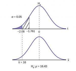
Step 4 has us compare the test statistic and the critical value and mark these on the graph. We see that the test statistic is in the tail and thus we move to step 4 and reach a conclusion. The probability that an average time of 16 minutes could come from a distribution with a population mean of 16.43 minutes is too unlikely for us to accept the null hypothesis. We cannot accept the null.

Step 5 has us state our conclusions first formally and then less formally. A formal conclusion would be stated as: “With a 95% level of significance we cannot accept the null hypothesis that the swimming time with goggles comes from a distribution with a population mean time of 16.43 minutes.” Less formally, “With 95% significance we believe that the goggles improves swimming speed”

If we wished to use the p-value system of reaching a conclusion we would calculate the statistic and take the additional step to find the probability of being 2.08 standard deviations from the mean on a t-distribution. This value is .0187. Comparing this to the α-level of .05 we see that we cannot accept the null. The p-value has been put on the graph as the shaded area beyond -2.08 and it shows that it is smaller than the hatched area which is the alpha level of 0.05. Both methods reach the same conclusion that we cannot accept the null hypothesis.

Jane has just begun her new job as on the sales force of a very competitive company. In a sample of 16 sales calls it was found that she closed the contract for an average value of $108 with a standard deviation of 12 dollars. Test at 5% significance that the population mean is at least $100 against the alternative that it is less than 100 dollars. Company policy requires that new members of the sales force must exceed an average of $100 per contract during the trial employment period. Can we conclude that Jane has met this requirement at the significance level of 95%?

Solution – Example 7

STEP 1 : Set the Null and Alternative Hypothesis.

STEP 2 : Decide the level of significance and draw the graph (Figure 7) showing the critical value.

STEP 3 : Calculate sample parameters and the test statistic.

STEP 4 : Compare test statistic and the critical values

STEP 5 : Reach a Conclusion

The test statistic is a Student’s t because the sample size is below 30; therefore, we cannot use the normal distribution. Comparing the calculated value of the test statistic and the critical value of t ( t a ) at a 5% significance level, we see that the calculated value is in the tail of the distribution. Thus, we conclude that 108 dollars per contract is significantly larger than the hypothesized value of 100 and thus we cannot accept the null hypothesis. There is evidence that supports Jane’s performance meets company standards.

Again we will follow the steps in our analysis of this problem.

Solution – Example 8

STEP 1 : Set the Null and Alternative Hypothesis. The random variable is the quantity of fluid placed in the bottles. This is a continuous random variable and the parameter we are interested in is the mean. Our hypothesis therefore is about the mean. In this case we are concerned that the machine is not filling properly. From what we are told it does not matter if the machine is over-filling or under-filling, both seem to be an equally bad error. This tells us that this is a two-tailed test: if the machine is malfunctioning it will be shutdown regardless if it is from over-filling or under-filling. The null and alternative hypotheses are thus:

STEP 2 : Decide the level of significance and draw the graph showing the critical value.

This problem has already set the level of significance at 99%. The decision seems an appropriate one and shows the thought process when setting the significance level. Management wants to be very certain, as certain as probability will allow, that they are not shutting down a machine that is not in need of repair. To draw the distribution and the critical value, we need to know which distribution to use. Because this is a continuous random variable and we are interested in the mean, and the sample size is greater than 30, the appropriate distribution is the normal distribution and the relevant critical value is 2.575 from the normal table or the t-table at 0.005 column and infinite degrees of freedom. We draw the graph and mark these points (Figure 8).

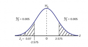
STEP 3 : Calculate sample parameters and the test statistic. The sample parameters are provided, the sample mean is 7.91 and the sample variance is .03 and the sample size is 35. We need to note that the sample variance was provided not the sample standard deviation, which is what we need for the formula. Remembering that the standard deviation is simply the square root of the variance, we therefore know the sample standard deviation, s, is 0.173. With this information we calculate the test statistic as -3.07, and mark it on the graph.

STEP 4 : Compare test statistic and the critical values Now we compare the test statistic and the critical value by placing the test statistic on the graph. We see that the test statistic is in the tail, decidedly greater than the critical value of 2.575. We note that even the very small difference between the hypothesized value and the sample value is still a large number of standard deviations. The sample mean is only 0.08 ounces different from the required level of 8 ounces, but it is 3 plus standard deviations away and thus we cannot accept the null hypothesis.

Three standard deviations of a test statistic will guarantee that the test will fail. The probability that anything is within three standard deviations is almost zero. Actually it is 0.0026 on the normal distribution, which is certainly almost zero in a practical sense. Our formal conclusion would be “ At a 99% level of significance we cannot accept the hypothesis that the sample mean came from a distribution with a mean of 8 ounces” Or less formally, and getting to the point, “At a 99% level of significance we conclude that the machine is under filling the bottles and is in need of repair”.

Media Attributions

• Type1Type2Error
• HypTestFig2
• HypTestFig3
• HypTestPValue
• OneTailTestFig5
• HypTestExam7
• HypTestExam8

Quantitative Analysis for Business Copyright © by Margo Bergman is licensed under a Creative Commons Attribution-NonCommercial-ShareAlike 4.0 International License , except where otherwise noted.

Share This Book

If you're seeing this message, it means we're having trouble loading external resources on our website.

If you're behind a web filter, please make sure that the domains *.kastatic.org and *.kasandbox.org are unblocked.

To log in and use all the features of Khan Academy, please enable JavaScript in your browser.

Statistics and probability

Course: statistics and probability   >   unit 12, simple hypothesis testing.

• Idea behind hypothesis testing
• Examples of null and alternative hypotheses
• Writing null and alternative hypotheses
• P-values and significance tests
• Comparing P-values to different significance levels
• Estimating a P-value from a simulation
• Estimating P-values from simulations
• Using P-values to make conclusions
• Your answer should be
• an integer, like 6 ‍  
• an exact decimal, like 0.75 ‍  
• a simplified proper fraction, like 3 / 5 ‍  
• a simplified improper fraction, like 7 / 4 ‍  
• a mixed number, like 1   3 / 4 ‍  
• a percent, like 12.34 % ‍  
• (Choice A)   We cannot reject the hypothesis. A We cannot reject the hypothesis.
• (Choice B)   We should reject the hypothesis. B We should reject the hypothesis.

Have a language expert improve your writing

Run a free plagiarism check in 10 minutes, generate accurate citations for free.

• Knowledge Base
• Choosing the Right Statistical Test | Types & Examples

Choosing the Right Statistical Test | Types & Examples

Published on January 28, 2020 by Rebecca Bevans . Revised on June 22, 2023.

Statistical tests are used in hypothesis testing . They can be used to:

• determine whether a predictor variable has a statistically significant relationship with an outcome variable.
• estimate the difference between two or more groups.

Statistical tests assume a null hypothesis of no relationship or no difference between groups. Then they determine whether the observed data fall outside of the range of values predicted by the null hypothesis.

If you already know what types of variables you’re dealing with, you can use the flowchart to choose the right statistical test for your data.

Statistical tests flowchart

Table of contents

What does a statistical test do, when to perform a statistical test, choosing a parametric test: regression, comparison, or correlation, choosing a nonparametric test, flowchart: choosing a statistical test, other interesting articles, frequently asked questions about statistical tests.

Statistical tests work by calculating a test statistic – a number that describes how much the relationship between variables in your test differs from the null hypothesis of no relationship.

It then calculates a p value (probability value). The p -value estimates how likely it is that you would see the difference described by the test statistic if the null hypothesis of no relationship were true.

If the value of the test statistic is more extreme than the statistic calculated from the null hypothesis, then you can infer a statistically significant relationship between the predictor and outcome variables.

If the value of the test statistic is less extreme than the one calculated from the null hypothesis, then you can infer no statistically significant relationship between the predictor and outcome variables.

Receive feedback on language, structure, and formatting

Professional editors proofread and edit your paper by focusing on:

• Academic style
• Vague sentences
• Style consistency

See an example

You can perform statistical tests on data that have been collected in a statistically valid manner – either through an experiment , or through observations made using probability sampling methods .

For a statistical test to be valid , your sample size needs to be large enough to approximate the true distribution of the population being studied.

To determine which statistical test to use, you need to know:

• whether your data meets certain assumptions.
• the types of variables that you’re dealing with.

Statistical assumptions

Statistical tests make some common assumptions about the data they are testing:

• Independence of observations (a.k.a. no autocorrelation): The observations/variables you include in your test are not related (for example, multiple measurements of a single test subject are not independent, while measurements of multiple different test subjects are independent).
• Homogeneity of variance : the variance within each group being compared is similar among all groups. If one group has much more variation than others, it will limit the test’s effectiveness.
• Normality of data : the data follows a normal distribution (a.k.a. a bell curve). This assumption applies only to quantitative data .

If your data do not meet the assumptions of normality or homogeneity of variance, you may be able to perform a nonparametric statistical test , which allows you to make comparisons without any assumptions about the data distribution.

If your data do not meet the assumption of independence of observations, you may be able to use a test that accounts for structure in your data (repeated-measures tests or tests that include blocking variables).

Types of variables

The types of variables you have usually determine what type of statistical test you can use.

Quantitative variables represent amounts of things (e.g. the number of trees in a forest). Types of quantitative variables include:

• Continuous (aka ratio variables): represent measures and can usually be divided into units smaller than one (e.g. 0.75 grams).
• Discrete (aka integer variables): represent counts and usually can’t be divided into units smaller than one (e.g. 1 tree).

Categorical variables represent groupings of things (e.g. the different tree species in a forest). Types of categorical variables include:

• Ordinal : represent data with an order (e.g. rankings).
• Nominal : represent group names (e.g. brands or species names).
• Binary : represent data with a yes/no or 1/0 outcome (e.g. win or lose).

Choose the test that fits the types of predictor and outcome variables you have collected (if you are doing an experiment , these are the independent and dependent variables ). Consult the tables below to see which test best matches your variables.

Parametric tests usually have stricter requirements than nonparametric tests, and are able to make stronger inferences from the data. They can only be conducted with data that adheres to the common assumptions of statistical tests.

The most common types of parametric test include regression tests, comparison tests, and correlation tests.

Regression tests

Regression tests look for cause-and-effect relationships . They can be used to estimate the effect of one or more continuous variables on another variable.

Comparison tests

Comparison tests look for differences among group means . They can be used to test the effect of a categorical variable on the mean value of some other characteristic.

T-tests are used when comparing the means of precisely two groups (e.g., the average heights of men and women). ANOVA and MANOVA tests are used when comparing the means of more than two groups (e.g., the average heights of children, teenagers, and adults).

Correlation tests

Correlation tests check whether variables are related without hypothesizing a cause-and-effect relationship.

These can be used to test whether two variables you want to use in (for example) a multiple regression test are autocorrelated.

Non-parametric tests don’t make as many assumptions about the data, and are useful when one or more of the common statistical assumptions are violated. However, the inferences they make aren’t as strong as with parametric tests.

Here's why students love Scribbr's proofreading services

Discover proofreading & editing

This flowchart helps you choose among parametric tests. For nonparametric alternatives, check the table above.

If you want to know more about statistics , methodology , or research bias , make sure to check out some of our other articles with explanations and examples.

• Normal distribution
• Descriptive statistics
• Measures of central tendency
• Correlation coefficient
• Null hypothesis

Methodology

• Cluster sampling
• Stratified sampling
• Types of interviews
• Cohort study
• Thematic analysis

Research bias

• Implicit bias
• Cognitive bias
• Survivorship bias
• Availability heuristic
• Nonresponse bias
• Regression to the mean

Statistical tests commonly assume that:

• the data are normally distributed
• the groups that are being compared have similar variance
• the data are independent

If your data does not meet these assumptions you might still be able to use a nonparametric statistical test , which have fewer requirements but also make weaker inferences.

A test statistic is a number calculated by a  statistical test . It describes how far your observed data is from the  null hypothesis  of no relationship between  variables or no difference among sample groups.

The test statistic tells you how different two or more groups are from the overall population mean , or how different a linear slope is from the slope predicted by a null hypothesis . Different test statistics are used in different statistical tests.

Statistical significance is a term used by researchers to state that it is unlikely their observations could have occurred under the null hypothesis of a statistical test . Significance is usually denoted by a p -value , or probability value.

Statistical significance is arbitrary – it depends on the threshold, or alpha value, chosen by the researcher. The most common threshold is p < 0.05, which means that the data is likely to occur less than 5% of the time under the null hypothesis .

When the p -value falls below the chosen alpha value, then we say the result of the test is statistically significant.

Quantitative variables are any variables where the data represent amounts (e.g. height, weight, or age).

Categorical variables are any variables where the data represent groups. This includes rankings (e.g. finishing places in a race), classifications (e.g. brands of cereal), and binary outcomes (e.g. coin flips).

You need to know what type of variables you are working with to choose the right statistical test for your data and interpret your results .

Discrete and continuous variables are two types of quantitative variables :

• Discrete variables represent counts (e.g. the number of objects in a collection).
• Continuous variables represent measurable amounts (e.g. water volume or weight).

Cite this Scribbr article

If you want to cite this source, you can copy and paste the citation or click the “Cite this Scribbr article” button to automatically add the citation to our free Citation Generator.

Bevans, R. (2023, June 22). Choosing the Right Statistical Test | Types & Examples. Scribbr. Retrieved March 29, 2024, from https://www.scribbr.com/statistics/statistical-tests/

Is this article helpful?

Rebecca Bevans

Other students also liked, hypothesis testing | a step-by-step guide with easy examples, test statistics | definition, interpretation, and examples, normal distribution | examples, formulas, & uses, what is your plagiarism score.

• Search Search Please fill out this field.
• Fundamental Analysis

Hypothesis to Be Tested: Definition and 4 Steps for Testing with Example

What Is Hypothesis Testing?

Hypothesis testing, sometimes called significance testing, is an act in statistics whereby an analyst tests an assumption regarding a population parameter. The methodology employed by the analyst depends on the nature of the data used and the reason for the analysis.

Hypothesis testing is used to assess the plausibility of a hypothesis by using sample data. Such data may come from a larger population, or from a data-generating process. The word "population" will be used for both of these cases in the following descriptions.

Key Takeaways

• Hypothesis testing is used to assess the plausibility of a hypothesis by using sample data.
• The test provides evidence concerning the plausibility of the hypothesis, given the data.
• Statistical analysts test a hypothesis by measuring and examining a random sample of the population being analyzed.
• The four steps of hypothesis testing include stating the hypotheses, formulating an analysis plan, analyzing the sample data, and analyzing the result.

How Hypothesis Testing Works

In hypothesis testing, an  analyst  tests a statistical sample, with the goal of providing evidence on the plausibility of the null hypothesis.

Statistical analysts test a hypothesis by measuring and examining a random sample of the population being analyzed. All analysts use a random population sample to test two different hypotheses: the null hypothesis and the alternative hypothesis.

The null hypothesis is usually a hypothesis of equality between population parameters; e.g., a null hypothesis may state that the population mean return is equal to zero. The alternative hypothesis is effectively the opposite of a null hypothesis (e.g., the population mean return is not equal to zero). Thus, they are mutually exclusive , and only one can be true. However, one of the two hypotheses will always be true.

The null hypothesis is a statement about a population parameter, such as the population mean, that is assumed to be true.

4 Steps of Hypothesis Testing

All hypotheses are tested using a four-step process:

• The first step is for the analyst to state the hypotheses.
• The second step is to formulate an analysis plan, which outlines how the data will be evaluated.
• The third step is to carry out the plan and analyze the sample data.
• The final step is to analyze the results and either reject the null hypothesis, or state that the null hypothesis is plausible, given the data.

Real-World Example of Hypothesis Testing

If, for example, a person wants to test that a penny has exactly a 50% chance of landing on heads, the null hypothesis would be that 50% is correct, and the alternative hypothesis would be that 50% is not correct.

Mathematically, the null hypothesis would be represented as Ho: P = 0.5. The alternative hypothesis would be denoted as "Ha" and be identical to the null hypothesis, except with the equal sign struck-through, meaning that it does not equal 50%.

A random sample of 100 coin flips is taken, and the null hypothesis is then tested. If it is found that the 100 coin flips were distributed as 40 heads and 60 tails, the analyst would assume that a penny does not have a 50% chance of landing on heads and would reject the null hypothesis and accept the alternative hypothesis.

If, on the other hand, there were 48 heads and 52 tails, then it is plausible that the coin could be fair and still produce such a result. In cases such as this where the null hypothesis is "accepted," the analyst states that the difference between the expected results (50 heads and 50 tails) and the observed results (48 heads and 52 tails) is "explainable by chance alone."

Some staticians attribute the first hypothesis tests to satirical writer John Arbuthnot in 1710, who studied male and female births in England after observing that in nearly every year, male births exceeded female births by a slight proportion. Arbuthnot calculated that the probability of this happening by chance was small, and therefore it was due to “divine providence.”

What is Hypothesis Testing?

Hypothesis testing refers to a process used by analysts to assess the plausibility of a hypothesis by using sample data. In hypothesis testing, statisticians formulate two hypotheses: the null hypothesis and the alternative hypothesis. A null hypothesis determines there is no difference between two groups or conditions, while the alternative hypothesis determines that there is a difference. Researchers evaluate the statistical significance of the test based on the probability that the null hypothesis is true.

What are the Four Key Steps Involved in Hypothesis Testing?

Hypothesis testing begins with an analyst stating two hypotheses, with only one that can be right. The analyst then formulates an analysis plan, which outlines how the data will be evaluated. Next, they move to the testing phase and analyze the sample data. Finally, the analyst analyzes the results and either rejects the null hypothesis or states that the null hypothesis is plausible, given the data.

What are the Benefits of Hypothesis Testing?

Hypothesis testing helps assess the accuracy of new ideas or theories by testing them against data. This allows researchers to determine whether the evidence supports their hypothesis, helping to avoid false claims and conclusions. Hypothesis testing also provides a framework for decision-making based on data rather than personal opinions or biases. By relying on statistical analysis, hypothesis testing helps to reduce the effects of chance and confounding variables, providing a robust framework for making informed conclusions.

What are the Limitations of Hypothesis Testing?

Hypothesis testing relies exclusively on data and doesn’t provide a comprehensive understanding of the subject being studied. Additionally, the accuracy of the results depends on the quality of the available data and the statistical methods used. Inaccurate data or inappropriate hypothesis formulation may lead to incorrect conclusions or failed tests. Hypothesis testing can also lead to errors, such as analysts either accepting or rejecting a null hypothesis when they shouldn’t have. These errors may result in false conclusions or missed opportunities to identify significant patterns or relationships in the data.

The Bottom Line

Hypothesis testing refers to a statistical process that helps researchers and/or analysts determine the reliability of a study. By using a well-formulated hypothesis and set of statistical tests, individuals or businesses can make inferences about the population that they are studying and draw conclusions based on the data presented. There are different types of hypothesis testing, each with their own set of rules and procedures. However, all hypothesis testing methods have the same four step process, which includes stating the hypotheses, formulating an analysis plan, analyzing the sample data, and analyzing the result. Hypothesis testing plays a vital part of the scientific process, helping to test assumptions and make better data-based decisions.

Sage. " Introduction to Hypothesis Testing. " Page 4.

Elder Research. " Who Invented the Null Hypothesis? "

Formplus. " Hypothesis Testing: Definition, Uses, Limitations and Examples. "

• Terms of Service
• Editorial Policy
• Privacy Policy
• Your Privacy Choices

Statistics Made Easy

Two Sample t-test: Definition, Formula, and Example

A two sample t-test is used to determine whether or not two population means are equal.

This tutorial explains the following:

• The motivation for performing a two sample t-test.
• The formula to perform a two sample t-test.
• The assumptions that should be met to perform a two sample t-test.
• An example of how to perform a two sample t-test.

Two Sample t-test: Motivation

Suppose we want to know whether or not the mean weight between two different species of turtles is equal. Since there are thousands of turtles in each population, it would be too time-consuming and costly to go around and weigh each individual turtle.

Instead, we might take a simple random sample of 15 turtles from each population and use the mean weight in each sample to determine if the mean weight is equal between the two populations:

However, it’s virtually guaranteed that the mean weight between the two samples will be at least a little different. The question is whether or not this difference is statistically significant . Fortunately, a two sample t-test allows us to answer this question.

Two Sample t-test: Formula

A two-sample t-test always uses the following null hypothesis:

• H 0 : μ 1  = μ 2 (the two population means are equal)

The alternative hypothesis can be either two-tailed, left-tailed, or right-tailed:

• H 1 (two-tailed): μ 1  ≠ μ 2 (the two population means are not equal)
• H 1 (left-tailed): μ 1  < μ 2  (population 1 mean is less than population 2 mean)
• H 1 (right-tailed):  μ 1 > μ 2  (population 1 mean is greater than population 2 mean)

We use the following formula to calculate the test statistic t:

Test statistic:  ( x 1  –  x 2 )  /  s p (√ 1/n 1  + 1/n 2 )

where  x 1  and  x 2 are the sample means, n 1 and n 2  are the sample sizes, and where s p is calculated as:

s p = √  (n 1 -1)s 1 2  +  (n 2 -1)s 2 2  /  (n 1 +n 2 -2)

where s 1 2  and s 2 2  are the sample variances.

If the p-value that corresponds to the test statistic t with (n 1 +n 2 -1) degrees of freedom is less than your chosen significance level (common choices are 0.10, 0.05, and 0.01) then you can reject the null hypothesis.

Two Sample t-test: Assumptions

For the results of a two sample t-test to be valid, the following assumptions should be met:

• The observations in one sample should be independent of the observations in the other sample.
• The data should be approximately normally distributed.
• The two samples should have approximately the same variance. If this assumption is not met, you should instead perform Welch’s t-test .
• The data in both samples was obtained using a random sampling method .

Two Sample t-test : Example

Suppose we want to know whether or not the mean weight between two different species of turtles is equal. To test this, will perform a two sample t-test at significance level α = 0.05 using the following steps:

Step 1: Gather the sample data.

Suppose we collect a random sample of turtles from each population with the following information:

• Sample size n 1 = 40
• Sample mean weight  x 1  = 300
• Sample standard deviation s 1 = 18.5
• Sample size n 2 = 38
• Sample mean weight  x 2  = 305
• Sample standard deviation s 2 = 16.7

Step 2: Define the hypotheses.

We will perform the two sample t-test with the following hypotheses:

• H 0 :  μ 1  = μ 2 (the two population means are equal)
• H 1 :  μ 1  ≠ μ 2 (the two population means are not equal)

Step 3: Calculate the test statistic  t .

First, we will calculate the pooled standard deviation s p :

s p = √  (n 1 -1)s 1 2  +  (n 2 -1)s 2 2  /  (n 1 +n 2 -2)  = √  (40-1)18.5 2  +  (38-1)16.7 2  /  (40+38-2)  = 17.647

Next, we will calculate the test statistic  t :

t = ( x 1  –  x 2 )  /  s p (√ 1/n 1  + 1/n 2 ) =  (300-305) / 17.647(√ 1/40 + 1/38 ) =  -1.2508

Step 4: Calculate the p-value of the test statistic  t .

According to the T Score to P Value Calculator , the p-value associated with t = -1.2508 and degrees of freedom = n 1 +n 2 -2 = 40+38-2 = 76 is  0.21484 .

Step 5: Draw a conclusion.

Since this p-value is not less than our significance level α = 0.05, we fail to reject the null hypothesis. We do not have sufficient evidence to say that the mean weight of turtles between these two populations is different.

Note:  You can also perform this entire two sample t-test by simply using the Two Sample t-test Calculator .

Additional Resources

The following tutorials explain how to perform a two-sample t-test using different statistical programs:

How to Perform a Two Sample t-test in Excel How to Perform a Two Sample t-test in SPSS How to Perform a Two Sample t-test in Stata How to Perform a Two Sample t-test in R How to Perform a Two Sample t-test in Python How to Perform a Two Sample t-test on a TI-84 Calculator

Published by Zach

Leave a reply cancel reply.

Your email address will not be published. Required fields are marked *

Help | Advanced Search

Mathematics > Statistics Theory

Title: the sample complexity of simple binary hypothesis testing.

Abstract: The sample complexity of simple binary hypothesis testing is the smallest number of i.i.d. samples required to distinguish between two distributions $p$ and $q$ in either: (i) the prior-free setting, with type-I error at most $\alpha$ and type-II error at most $\beta$; or (ii) the Bayesian setting, with Bayes error at most $\delta$ and prior distribution $(\alpha, 1-\alpha)$. This problem has only been studied when $\alpha = \beta$ (prior-free) or $\alpha = 1/2$ (Bayesian), and the sample complexity is known to be characterized by the Hellinger divergence between $p$ and $q$, up to multiplicative constants. In this paper, we derive a formula that characterizes the sample complexity (up to multiplicative constants that are independent of $p$, $q$, and all error parameters) for: (i) all $0 \le \alpha, \beta \le 1/8$ in the prior-free setting; and (ii) all $\delta \le \alpha/4$ in the Bayesian setting. In particular, the formula admits equivalent expressions in terms of certain divergences from the Jensen--Shannon and Hellinger families. The main technical result concerns an $f$-divergence inequality between members of the Jensen--Shannon and Hellinger families, which is proved by a combination of information-theoretic tools and case-by-case analyses. We explore applications of our results to robust and distributed (locally-private and communication-constrained) hypothesis testing.

Submission history

Access paper:.

• HTML (experimental)
• Other Formats

References & Citations

• Google Scholar
• Semantic Scholar

BibTeX formatted citation

Bibliographic and Citation Tools

Code, data and media associated with this article, recommenders and search tools.

• Institution

arXivLabs: experimental projects with community collaborators

arXivLabs is a framework that allows collaborators to develop and share new arXiv features directly on our website.

Both individuals and organizations that work with arXivLabs have embraced and accepted our values of openness, community, excellence, and user data privacy. arXiv is committed to these values and only works with partners that adhere to them.

Have an idea for a project that will add value for arXiv's community? Learn more about arXivLabs .

• school Campus Bookshelves
• menu_book Bookshelves
• perm_media Learning Objects
• login Login
• how_to_reg Request Instructor Account
• hub Instructor Commons
• Download Page (PDF)
• Download Full Book (PDF)
• Periodic Table
• Physics Constants
• Scientific Calculator
• Reference & Cite
• Tools expand_more
• Readability

selected template will load here

This action is not available.

8.4: Hypothesis Test Examples for Proportions

• Last updated
• Save as PDF
• Page ID 11533

• In a hypothesis test problem, you may see words such as "the level of significance is 1%." The "1%" is the preconceived or preset \(\alpha\).
• The statistician setting up the hypothesis test selects the value of α to use before collecting the sample data.
• If no level of significance is given, a common standard to use is \(\alpha = 0.05\).
• When you calculate the \(p\)-value and draw the picture, the \(p\)-value is the area in the left tail, the right tail, or split evenly between the two tails. For this reason, we call the hypothesis test left, right, or two tailed.
• The alternative hypothesis, \(H_{a}\), tells you if the test is left, right, or two-tailed. It is the key to conducting the appropriate test.
• \(H_{a}\) never has a symbol that contains an equal sign.
• Thinking about the meaning of the \(p\)-value: A data analyst (and anyone else) should have more confidence that he made the correct decision to reject the null hypothesis with a smaller \(p\)-value (for example, 0.001 as opposed to 0.04) even if using the 0.05 level for alpha. Similarly, for a large p -value such as 0.4, as opposed to a \(p\)-value of 0.056 (\(\alpha = 0.05\) is less than either number), a data analyst should have more confidence that she made the correct decision in not rejecting the null hypothesis. This makes the data analyst use judgment rather than mindlessly applying rules.

Full Hypothesis Test Examples

Example \(\PageIndex{7}\)

Joon believes that 50% of first-time brides in the United States are younger than their grooms. She performs a hypothesis test to determine if the percentage is the same or different from 50% . Joon samples 100 first-time brides and 53 reply that they are younger than their grooms. For the hypothesis test, she uses a 1% level of significance.

Set up the hypothesis test:

The 1% level of significance means that α = 0.01. This is a test of a single population proportion .

\(H_{0}: p = 0.50\)  \(H_{a}: p \neq 0.50\)

The words "is the same or different from" tell you this is a two-tailed test.

Calculate the distribution needed:

Random variable: \(P′ =\) the percent of of first-time brides who are younger than their grooms.

Distribution for the test: The problem contains no mention of a mean. The information is given in terms of percentages. Use the distribution for P′ , the estimated proportion.

\[P' - N\left(p, \sqrt{\frac{p-q}{n}}\right)\nonumber \]

\[P' - N\left(0.5, \sqrt{\frac{0.5-0.5}{100}}\right)\nonumber \]

where \(p = 0.50, q = 1−p = 0.50\), and \(n = 100\)

Calculate the p -value using the normal distribution for proportions:

\[p\text{-value} = P(p′ < 0.47 or p′ > 0.53) = 0.5485\nonumber \]

where \[x = 53, p' = \frac{x}{n} = \frac{53}{100} = 0.53\nonumber \].

Interpretation of the \(p\text{-value})\: If the null hypothesis is true, there is 0.5485 probability (54.85%) that the sample (estimated) proportion \(p'\) is 0.53 or more OR 0.47 or less (see the graph in Figure).

\(\mu = p = 0.50\) comes from \(H_{0}\), the null hypothesis.

\(p′ = 0.53\). Since the curve is symmetrical and the test is two-tailed, the \(p′\) for the left tail is equal to \(0.50 – 0.03 = 0.47\) where \(\mu = p = 0.50\). (0.03 is the difference between 0.53 and 0.50.)

Compare \(\alpha\) and the \(p\text{-value}\):

Since \(\alpha = 0.01\) and \(p\text{-value} = 0.5485\). \(\alpha < p\text{-value}\).

Make a decision: Since \(\alpha < p\text{-value}\), you cannot reject \(H_{0}\).

Conclusion: At the 1% level of significance, the sample data do not show sufficient evidence that the percentage of first-time brides who are younger than their grooms is different from 50%.

The \(p\text{-value}\) can easily be calculated.

Press STAT and arrow over to TESTS . Press 5:1-PropZTest . Enter .5 for \(p_{0}\), 53 for \(x\) and 100 for \(n\). Arrow down to Prop and arrow to not equals \(p_{0}\). Press ENTER . Arrow down to Calculate and press ENTER . The calculator calculates the \(p\text{-value}\) (\(p = 0.5485\)) and the test statistic (\(z\)-score). Prop not equals .5 is the alternate hypothesis. Do this set of instructions again except arrow to Draw (instead of Calculate ). Press ENTER . A shaded graph appears with \(\(z\) = 0.6\) (test statistic) and \(p = 0.5485\) (\(p\text{-value}\)). Make sure when you use Draw that no other equations are highlighted in \(Y =\) and the plots are turned off.

The Type I and Type II errors are as follows:

The Type I error is to conclude that the proportion of first-time brides who are younger than their grooms is different from 50% when, in fact, the proportion is actually 50%. (Reject the null hypothesis when the null hypothesis is true).

The Type II error is there is not enough evidence to conclude that the proportion of first time brides who are younger than their grooms differs from 50% when, in fact, the proportion does differ from 50%. (Do not reject the null hypothesis when the null hypothesis is false.)

Exercise \(\PageIndex{7}\)

A teacher believes that 85% of students in the class will want to go on a field trip to the local zoo. She performs a hypothesis test to determine if the percentage is the same or different from 85%. The teacher samples 50 students and 39 reply that they would want to go to the zoo. For the hypothesis test, use a 1% level of significance.

First, determine what type of test this is, set up the hypothesis test, find the \(p\text{-value}\), sketch the graph, and state your conclusion.

Since the problem is about percentages, this is a test of single population proportions.

• \(H_{0} : p = 0.85\)
• \(H_{a}: p \neq 0.85\)
• \(p = 0.7554\)

Because \(p > \alpha\), we fail to reject the null hypothesis. There is not sufficient evidence to suggest that the proportion of students that want to go to the zoo is not 85%.

Example \(\PageIndex{8}\)

Suppose a consumer group suspects that the proportion of households that have three cell phones is 30%. A cell phone company has reason to believe that the proportion is not 30%. Before they start a big advertising campaign, they conduct a hypothesis test. Their marketing people survey 150 households with the result that 43 of the households have three cell phones.

Set up the Hypothesis Test:

\(H_{0}: p = 0.30, H_{a}: p \neq 0.30\)

Determine the distribution needed:

The random variable is \(P′ =\) proportion of households that have three cell phones.

The distribution for the hypothesis test is \(P' - N\left(0.30, \sqrt{\frac{(0.30 \cdot 0.70)}{150}}\right)\)

Exercise 9.6.8.2

a. The value that helps determine the \(p\text{-value}\) is \(p′\). Calculate \(p′\).

a. \(p' = \frac{x}{n}\) where \(x\) is the number of successes and \(n\) is the total number in the sample.

\(x = 43, n = 150\)

\(p′ = 43150\)

Exercise 9.6.8.3

b. What is a success for this problem?

b. A success is having three cell phones in a household.

Exercise 9.6.8.4

c. What is the level of significance?

c. The level of significance is the preset \(\alpha\). Since \(\alpha\) is not given, assume that \(\alpha = 0.05\).

Exercise 9.6.8.5

d. Draw the graph for this problem. Draw the horizontal axis. Label and shade appropriately.

Calculate the \(p\text{-value}\).

d. \(p\text{-value} = 0.7216\)

Exercise 9.6.8.6

e. Make a decision. _____________(Reject/Do not reject) \(H_{0}\) because____________.

e. Assuming that \(\alpha = 0.05, \alpha < p\text{-value}\). The decision is do not reject \(H_{0}\) because there is not sufficient evidence to conclude that the proportion of households that have three cell phones is not 30%.

Exercise \(\PageIndex{8}\)

Marketers believe that 92% of adults in the United States own a cell phone. A cell phone manufacturer believes that number is actually lower. 200 American adults are surveyed, of which, 174 report having cell phones. Use a 5% level of significance. State the null and alternative hypothesis, find the p -value, state your conclusion, and identify the Type I and Type II errors.

• \(H_{0}: p = 0.92\)
• \(H_{a}: p < 0.92\)
• \(p\text{-value} = 0.0046\)

Because \(p < 0.05\), we reject the null hypothesis. There is sufficient evidence to conclude that fewer than 92% of American adults own cell phones.

• Type I Error: To conclude that fewer than 92% of American adults own cell phones when, in fact, 92% of American adults do own cell phones (reject the null hypothesis when the null hypothesis is true).
• Type II Error: To conclude that 92% of American adults own cell phones when, in fact, fewer than 92% of American adults own cell phones (do not reject the null hypothesis when the null hypothesis is false).

The next example is a poem written by a statistics student named Nicole Hart. The solution to the problem follows the poem. Notice that the hypothesis test is for a single population proportion. This means that the null and alternate hypotheses use the parameter \(p\). The distribution for the test is normal. The estimated proportion \(p′\) is the proportion of fleas killed to the total fleas found on Fido. This is sample information. The problem gives a preconceived \(\alpha = 0.01\), for comparison, and a 95% confidence interval computation. The poem is clever and humorous, so please enjoy it!

Example \(\PageIndex{9}\)

My dog has so many fleas,

They do not come off with ease. As for shampoo, I have tried many types Even one called Bubble Hype, Which only killed 25% of the fleas, Unfortunately I was not pleased.

I've used all kinds of soap, Until I had given up hope Until one day I saw An ad that put me in awe.

A shampoo used for dogs Called GOOD ENOUGH to Clean a Hog Guaranteed to kill more fleas.

I gave Fido a bath And after doing the math His number of fleas Started dropping by 3's! Before his shampoo I counted 42.

At the end of his bath, I redid the math And the new shampoo had killed 17 fleas. So now I was pleased.

Now it is time for you to have some fun With the level of significance being .01, You must help me figure out

Use the new shampoo or go without?

\(H_{0}: p \leq 0.25\)   \(H_{a}: p > 0.25\)

In words, CLEARLY state what your random variable \(\bar{X}\) or \(P′\) represents.

\(P′ =\) The proportion of fleas that are killed by the new shampoo

State the distribution to use for the test.

\[N\left(0.25, \sqrt{\frac{(0.25){1-0.25}}{42}}\right)\nonumber \]

Test Statistic: \(z = 2.3163\)

Calculate the \(p\text{-value}\) using the normal distribution for proportions:

\[p\text{-value} = 0.0103\nonumber \]

In one to two complete sentences, explain what the p -value means for this problem.

If the null hypothesis is true (the proportion is 0.25), then there is a 0.0103 probability that the sample (estimated) proportion is 0.4048 \(\left(\frac{17}{42}\right)\) or more.

Use the previous information to sketch a picture of this situation. CLEARLY, label and scale the horizontal axis and shade the region(s) corresponding to the \(p\text{-value}\).

Indicate the correct decision (“reject” or “do not reject” the null hypothesis), the reason for it, and write an appropriate conclusion, using complete sentences.

Conclusion: At the 1% level of significance, the sample data do not show sufficient evidence that the percentage of fleas that are killed by the new shampoo is more than 25%.

Construct a 95% confidence interval for the true mean or proportion. Include a sketch of the graph of the situation. Label the point estimate and the lower and upper bounds of the confidence interval.

Confidence Interval: (0.26,0.55) We are 95% confident that the true population proportion p of fleas that are killed by the new shampoo is between 26% and 55%.

This test result is not very definitive since the \(p\text{-value}\) is very close to alpha. In reality, one would probably do more tests by giving the dog another bath after the fleas have had a chance to return.

Example \(\PageIndex{11}\)

In a study of 420,019 cell phone users, 172 of the subjects developed brain cancer. Test the claim that cell phone users developed brain cancer at a greater rate than that for non-cell phone users (the rate of brain cancer for non-cell phone users is 0.0340%). Since this is a critical issue, use a 0.005 significance level. Explain why the significance level should be so low in terms of a Type I error.

We will follow the four-step process.

• \(H_{0}: p \leq 0.00034\)
• \(H_{a}: p > 0.00034\)

If we commit a Type I error, we are essentially accepting a false claim. Since the claim describes cancer-causing environments, we want to minimize the chances of incorrectly identifying causes of cancer.

• We will be testing a sample proportion with \(x = 172\) and \(n = 420,019\). The sample is sufficiently large because we have \(np = 420,019(0.00034) = 142.8\), \(nq = 420,019(0.99966) = 419,876.2\), two independent outcomes, and a fixed probability of success \(p = 0.00034\). Thus we will be able to generalize our results to the population.

Figure 9.6.11.

Figure 9.6.12.

• Since the \(p\text{-value} = 0.0073\) is greater than our alpha value \(= 0.005\), we cannot reject the null. Therefore, we conclude that there is not enough evidence to support the claim of higher brain cancer rates for the cell phone users.

Example \(\PageIndex{12}\)

According to the US Census there are approximately 268,608,618 residents aged 12 and older. Statistics from the Rape, Abuse, and Incest National Network indicate that, on average, 207,754 rapes occur each year (male and female) for persons aged 12 and older. This translates into a percentage of sexual assaults of 0.078%. In Daviess County, KY, there were reported 11 rapes for a population of 37,937. Conduct an appropriate hypothesis test to determine if there is a statistically significant difference between the local sexual assault percentage and the national sexual assault percentage. Use a significance level of 0.01.

We will follow the four-step plan.

• We need to test whether the proportion of sexual assaults in Daviess County, KY is significantly different from the national average.
• \(H_{0}: p = 0.00078\)
• \(H_{a}: p \neq 0.00078\)

Figure 9.6.13.

Figure 9.6.14.

• Since the \(p\text{-value}\), \(p = 0.00063\), is less than the alpha level of 0.01, the sample data indicates that we should reject the null hypothesis. In conclusion, the sample data support the claim that the proportion of sexual assaults in Daviess County, Kentucky is different from the national average proportion.

The hypothesis test itself has an established process. This can be summarized as follows:

• Determine \(H_{0}\) and \(H_{a}\). Remember, they are contradictory.
• Determine the random variable.
• Determine the distribution for the test.
• Draw a graph, calculate the test statistic, and use the test statistic to calculate the \(p\text{-value}\). (A z -score and a t -score are examples of test statistics.)
• Compare the preconceived α with the p -value, make a decision (reject or do not reject H 0 ), and write a clear conclusion using English sentences.

Notice that in performing the hypothesis test, you use \(\alpha\) and not \(\beta\). \(\beta\) is needed to help determine the sample size of the data that is used in calculating the \(p\text{-value}\). Remember that the quantity \(1 – \beta\) is called the Power of the Test . A high power is desirable. If the power is too low, statisticians typically increase the sample size while keeping α the same.If the power is low, the null hypothesis might not be rejected when it should be.

• Data from Amit Schitai. Director of Instructional Technology and Distance Learning. LBCC.
• Data from Bloomberg Businessweek . Available online at http://www.businessweek.com/news/2011- 09-15/nyc-smoking-rate-falls-to-record-low-of-14-bloomberg-says.html.
• Data from energy.gov. Available online at http://energy.gov (accessed June 27. 2013).
• Data from Gallup®. Available online at www.gallup.com (accessed June 27, 2013).
• Data from Growing by Degrees by Allen and Seaman.
• Data from La Leche League International. Available online at www.lalecheleague.org/Law/BAFeb01.html.
• Data from the American Automobile Association. Available online at www.aaa.com (accessed June 27, 2013).
• Data from the American Library Association. Available online at www.ala.org (accessed June 27, 2013).
• Data from the Bureau of Labor Statistics. Available online at http://www.bls.gov/oes/current/oes291111.htm .
• Data from the Centers for Disease Control and Prevention. Available online at www.cdc.gov (accessed June 27, 2013)
• Data from the U.S. Census Bureau, available online at quickfacts.census.gov/qfd/states/00000.html (accessed June 27, 2013).
• Data from the United States Census Bureau. Available online at www.census.gov/hhes/socdemo/language/.
• Data from Toastmasters International. Available online at http://toastmasters.org/artisan/deta...eID=429&Page=1 .
• Data from Weather Underground. Available online at www.wunderground.com (accessed June 27, 2013).
• Federal Bureau of Investigations. “Uniform Crime Reports and Index of Crime in Daviess in the State of Kentucky enforced by Daviess County from 1985 to 2005.” Available online at http://www.disastercenter.com/kentucky/crime/3868.htm (accessed June 27, 2013).
• “Foothill-De Anza Community College District.” De Anza College, Winter 2006. Available online at research.fhda.edu/factbook/DA...t_da_2006w.pdf.
• Johansen, C., J. Boice, Jr., J. McLaughlin, J. Olsen. “Cellular Telephones and Cancer—a Nationwide Cohort Study in Denmark.” Institute of Cancer Epidemiology and the Danish Cancer Society, 93(3):203-7. Available online at http://www.ncbi.nlm.nih.gov/pubmed/11158188 (accessed June 27, 2013).
• Rape, Abuse & Incest National Network. “How often does sexual assault occur?” RAINN, 2009. Available online at www.rainn.org/get-information...sexual-assault (accessed June 27, 2013).

Contributors and Attributions

Barbara Illowsky and Susan Dean (De Anza College) with many other contributing authors. Content produced by OpenStax College is licensed under a Creative Commons Attribution License 4.0 license. Download for free at http://cnx.org/contents/[email protected] .