5.2 assignment vector components

school Campus Bookshelves
menu_book Bookshelves
perm_media Learning Objects
login Login
how_to_reg Request Instructor Account
hub Instructor Commons
Download Page (PDF)
Download Full Book (PDF)
Periodic Table
Physics Constants
Scientific Calculator
Reference & Cite
Tools expand_more
Readability

selected template will load here

This action is not available.

1.5: Resolving Vectors into Components

Last updated
Save as PDF
Page ID 2813

Resolving Vectors into Axial Components

We know that when two vectors are in the same dimension, they can be added arithmetically. Suppose we have two vectors that are on a north-south, east-west grid, as shown below. One of the methods we can use to add these vectors is to resolve each one into a pair of vectors that lay on the north-south and east-west axes.

The two vectors we are to add is a force of 65 N at 30° north of east and a force of 35 N at 60° north of west.

We can resolve each of the vectors into two components on the axes lines. Each vector is resolved into a component on the north-south axis and a component on the east-west axis.

Using trigonometry, we can resolve (break down) each of these vectors into a pair of vectors that lay on the axial lines (shown in red above).

The east-west component of the first vector is (65 N)(cos 30° ) = (65 N)(0.866) = 56.3 N east

The north-south component of the first vector is (65 N)(sin 30°) = (65 N)(0.500) = 32.5 N north

The east-west component of the 2 nd vector is (35 N)(cos 60°) = (35 N)(0.500) = 17.5 N west

The north-south component of the 2 nd vector is (35 N)(sin 60°) = (35 N)(0.866) = 30.3 N north

Explore how to resolve vectors into axial components by hanging portraits of legendary physicists in the simulation below. The angle of each string determines how its tension force is distributed in both the horizontal and vertical dimensions. Under what conditions will the strings holding the portrait snap?

Interactive Element

Vectors can be resolved into component vectors that lie on the axes lines.
A force of 150. N is exerted 22° north of east. Find the northward and eastward components of this force.
An automobile travels a displacement of 75 km 45° north of east. How far east does it travel and how far north does it travel?

Explore More

Use this resource to answer the questions that follow.

What does SohCahToa mean?
Why is SohCahToa relevant to resolving a vector into components?
Why is the sum of the components larger than the resultant vector?

Additional Resources

Real World Application: Physics Behind Darts

PLIX: Play, Learn, Interact, eXplore: Bow and Arrow

school Campus Bookshelves
menu_book Bookshelves
perm_media Learning Objects
login Login
how_to_reg Request Instructor Account
hub Instructor Commons
Download Page (PDF)
Download Full Book (PDF)
Periodic Table
Physics Constants
Scientific Calculator
Reference & Cite
Tools expand_more
Readability

selected template will load here

This action is not available.

2.5: Coordinate Systems and Components of a Vector (Part 2)

Last updated
Save as PDF
Page ID 3974

Polar Coordinates

To describe locations of points or vectors in a plane, we need two orthogonal directions. In the Cartesian coordinate system these directions are given by unit vectors $\hat{i}$ and $\hat{j}$ along the x-axis and the y-axis, respectively. The Cartesian coordinate system is very convenient to use in describing displacements and velocities of objects and the forces acting on them. However, it becomes cumbersome when we need to describe the rotation of objects. When describing rotation, we usually work in the polar coordinate system .

In the polar coordinate system, the location of point P in a plane is given by two polar coordinates (Figure $\PageIndex{1}$). The first polar coordinate is the radial coordinate r, which is the distance of point P from the origin. The second polar coordinate is an angle $\varphi$ that the radial vector makes with some chosen direction, usually the positive x-direction. In polar coordinates, angles are measured in radians, or rads. The radial vector is attached at the origin and points away from the origin to point P. This radial direction is described by a unit radial vector $\hat{r}$. The second unit vector $\hat{t}$ is a vector orthogonal to the radial direction $\hat{r}$. The positive + $\hat{t}$ direction indicates how the angle $\varphi$ changes in the counterclockwise direction. In this way, a point P that has coordinates (x, y) in the rectangular system can be described equivalently in the polar coordinate system by the two polar coordinates (r, $\varphi$). Equation 2.4.13 is valid for any vector, so we can use it to express the x- and y-coordinates of vector $\vec{r}$. In this way, we obtain the connection between the polar coordinates and rectangular coordinates of point P:

\[ \begin{cases} x = r \cos \varphi \\ y = r \sin \varphi \end{cases} \ldotp \label{2.18}\]

Vector r points from the origin of the x y coordinate system to point P. The angle between the vector r and the positive x direction is phi. X equals r cosine phi and y equals r sine phi. Extending a line in the direction of r vector past point P, a unit vector r hat is drawn in the same direction as r. A unit vector t hat is perpendicular to r hat, pointing 90 degrees counterclockwise to r hat.

Example $\PageIndex{1}$: Polar Coordinates

A treasure hunter finds one silver coin at a location 20.0 m away from a dry well in the direction 20° north of east and finds one gold coin at a location 10.0 m away from the well in the direction 20° north of west. What are the polar and rectangular coordinates of these findings with respect to the well?

The well marks the origin of the coordinate system and east is the +x-direction. We identify radial distances from the locations to the origin, which are r S = 20.0 m (for the silver coin) and r G = 10.0 m (for the gold coin). To find the angular coordinates, we convert 20° to radians: 20° = $\frac{\pi\; 20}{180}$ = $\frac{\pi}{9}$. We use Equation \ref{2.18} to find the x- and y-coordinates of the coins.

The angular coordinate of the silver coin is $\varphi_{S}$ = $\frac{\pi}{9}$, whereas the angular coordinate of the gold coin is $\varphi_{G}$ = $\pi$ − $\frac{\pi}{9}$ = $\frac{8 \pi}{9}$. Hence, the polar coordinates of the silver coin are (r S , $\varphi_{S}$) = (20.0 m, $\frac{\pi}{9}$) and those of the gold coin are (r G , $\varphi_{G}$) = (10.0 m, \frac{8 \pi}{9}\)). We substitute these coordinates into Equation \ref{2.18} to obtain rectangular coordinates. For the gold coin, the coordinates are

\[ \begin{cases} x_{G} = r_{G} \cos \varphi_{G} = (10.0\; m) \cos \frac{8 \pi}{9} = -9.4\; m \\ y_{G} = r_{G} \sin \varphi_{G} = (10.0\; m) \sin \frac{8 \pi}{9} = 3.4\; m \end{cases} \Rightarrow (x_{G}, y_{G}) = (-9.4\; m, 3.4\; m) \ldotp\]

For the silver coin, the coordinates are

\[ \begin{cases} x_{S} = r_{S} \cos \varphi_{S} = (20.0\; m) \cos \frac{\pi}{9} = 18.9\; m \\ y_{S} = r_{S} \sin \varphi_{S} = (20.0\; m) \sin \frac{\pi}{9} = 6.8\; m \end{cases} \Rightarrow (x_{S}, y_{S}) = (18.9\; m, 6.8\; m) \ldotp\]

Vectors in Three Dimensions

To specify the location of a point in space, we need three coordinates (x, y, z), where coordinates x and y specify locations in a plane, and coordinate z gives a vertical positions above or below the plane. Three-dimensional space has three orthogonal directions, so we need not two but three unit vectors to define a three-dimensional coordinate system. In the Cartesian coordinate system, the first two unit vectors are the unit vector of the x-axis $\hat{i}$ and the unit vector of the y-axis $\hat{j}$. The third unit vector $\hat{k}$ is the direction of the z-axis (Figure $\PageIndex{2}$). The order in which the axes are labeled, which is the order in which the three unit vectors appear, is important because it defines the orientation of the coordinate system. The order x-y-z, which is equivalent to the order $\hat{i}$ - $\hat{j}$ - $\hat{k}$, defines the standard right-handed coordinate system (positive orientation).

The x y z coordinate system, with unit vectors I hat, j hat and k hat respectively. I hat points out at us, j hat points to the right, and k hat points up the page. The unit vectors form the sides of a cube.

In three-dimensional space, vector $\vec{A}$ has three vector components: the x-component $\vec{A}_{x}$ = A x $\hat{i}$, which is the part of vector $\vec{A}$ along the x-axis; the y-component $\vec{A}_{y}$ = A y $\hat{j}$, which is the part of $\vec{A}$ along the y-axis; and the z-component $\vec{A}_{z}$ = A z $\hat{k}$, which is the part of the vector along the z-axis. A vector in three-dimensional space is the vector sum of its three vector components (Figure $\PageIndex{3}$):

\[\vec{A} = A_{x} \hat{i} + A_{y} \hat{j} + A_{z} \hat{k} \ldotp \label{2.19}\]

If we know the coordinates of its origin b(x b , y b , z b ) and of its end e(x e y e , z e ), its scalar components are obtained by taking their differences: A x and A y are given by

\[ \begin{cases} A_{x} = x_{e} - x_{b} \nonumber \\ A_{y} = y_{e} - y_{b} \ldotp \nonumber \end{cases} \]

and the z-component is given by

\[A_{z} = z_{e} - z_{b} \ldotp \label{2.20}\]

Magnitude A is obtained by generalizing Equation 2.4.8 to three dimensions:

\[A = \sqrt{A_{x}^{2} + A_{y}^{2} + A_{z}^{2}} \ldotp \label{2.21}\]

This expression for the vector magnitude comes from applying the Pythagorean theorem twice. As seen in Figure $\PageIndex{3}$, the diagonal in the xy-plane has length $\sqrt{A_{x}^{2} + A_{y}^{2}}$ and its square adds to the square A z 2 to give A 2 . Note that when the z-component is zero, the vector lies entirely in the xy-plane and its description is reduced to two dimensions.

Vector A in the x y z coordinate system extends from the origin. Vector A equals the sum of vectors A sub x, A sub y and A sub z. Vector A sub x is the x component along the x axis and has length A sub x I hat. Vector A sub y is the y component along the y axis and has length A sub y j hat. Vector A sub z is the z component along the z axis and has length A sub x k hat. The components form the sides of a rectangular box with sides length A sub x, A sub y, and A sub z.

Example $\PageIndex{2}$: Takeoff of a Drone

During a takeoff of IAI Heron (Figure $\PageIndex{4}$), its position with respect to a control tower is 100 m above the ground, 300 m to the east, and 200 m to the north. One minute later, its position is 250 m above the ground, 1200 m to the east, and 2100 m to the north. What is the drone’s displacement vector with respect to the control tower? What is the magnitude of its displacement vector?

We take the origin of the Cartesian coordinate system as the control tower. The direction of the +x-axis is given by unit vector $\hat{i}$ to the east, the direction of the +y-axis is given by unit vector $\hat{j}$ to the north, and the direction of the +z-axis is given by unit vector $\hat{k}$, which points up from the ground. The drone’s first position is the origin (or, equivalently, the beginning) of the displacement vector and its second position is the end of the displacement vector.

We identify b(300.0 m, 200.0 m, 100.0 m) and e(480.0 m, 370.0 m, 250.0m), and use Equation 2.4.4 and Equation \ref{2.20} to find the scalar components of the drone’s displacement vector:

\[ \begin{cases} D_{x} = x_{e} - x_{b} = 1200.0\; m - 300.0\; m = 900.0\; m,\\ D_{y} =y_{e} - y_{b} = 2100.0\; m - 200.0\; m = 1900.0\; m, \\ D_{z} =z_{e} - z_{b} = 250.0\; m - 100.0\; m = 150\; m \ldotp \end{cases}\]

We substitute these components into Equation \ref{2.19} to find the displacement vector:

\[\vec{D} = D_{x}\; \hat{i} + D_{y}\; \hat{j} + D_{z}\; \hat{k} = 900.0\; \hat{i} + 1900.0\; \hat{j} + 150.0\; \hat{k} = (0.90\; \hat{i} + 1.90\; \hat{j} + 0.15\; \hat{k})\; km \ldotp\]

We substitute into Equation \ref{2.21} to find the magnitude of the displacement:

\[D = \sqrt{D_{x}^{2} + D_{y}^{2} + D_{z}^{2}} = \sqrt{(0.90\; km)^{2} + (1.90\; km)^{2} + (0.15\; km)^{2}} = 4.44\; km \ldotp\]

Exercise 2.7

If the average velocity vector of the drone in the displacement in Example 2.7 is $\vec{u}$ = (15.0 $\hat{i}$ + 31.7 $\hat{j}$ + 2.5 $\hat{k}$) m/s, what is the magnitude of the drone’s velocity vector?

5.2 Vector Addition and Subtraction: Analytical Methods

Learning objectives.

By the end of this section, you will be able to do the following:

Define components of vectors
Describe the analytical method of vector addition and subtraction
Use the analytical method of vector addition and subtraction to solve problems

Components of Vectors

For the analytical method of vector addition and subtraction, we use some simple geometry and trigonometry, instead of using a ruler and protractor as we did for graphical methods. However, the graphical method will still come in handy to visualize the problem by drawing vectors using the head-to-tail method. The analytical method is more accurate than the graphical method, which is limited by the precision of the drawing. For a refresher on the definitions of the sine, cosine, and tangent of an angle, see Figure 5.18 .

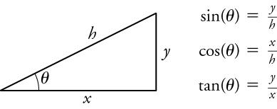
A right triangle is shown. The hypotenuse is labeled h, the vertical leg is labeled Y, and the horizontal leg is labeled X. The right angle is labeled with the angle symbol. The following formulas appear next to the triangle: sine angle equals y over h, cosine angle equals x over h, and tangent angle equals y over x.

Since, by definition, cos θ = x / h cos θ = x / h , we can find the length x if we know h and θ θ by using x = h cos θ x = h cos θ . Similarly, we can find the length of y by using y = h sin θ y = h sin θ . These trigonometric relationships are useful for adding vectors.

When a vector acts in more than one dimension, it is useful to break it down into its x and y components. For a two-dimensional vector, a component is a piece of a vector that points in either the x- or y-direction. Every 2-d vector can be expressed as a sum of its x and y components.

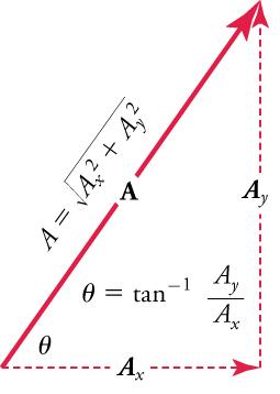
For example, given a vector like A A in Figure 5.19 , we may want to find what two perpendicular vectors, A x A x and A y A y , add to produce it. In this example, A x A x and A y A y form a right triangle, meaning that the angle between them is 90 degrees. This is a common situation in physics and happens to be the least complicated situation trigonometrically.

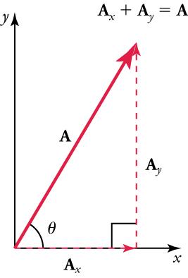
Vectors A, Ax, and Ay are shown. The vector A, with its tail at the origin of an x, y-coordinate system, is shown together with its x- and y-components, Ax and Ay. These vectors form a right triangle. The formula Ax plus Ay equals A is shown above the vectors.

A x A x and A y A y are defined to be the components of A A along the x - and y -axes. The three vectors, A A , A x A x , and A y A y , form a right triangle.

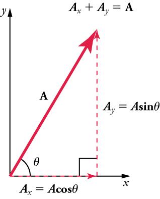
If the vector A A is known, then its magnitude A A (its length) and its angle θ θ (its direction) are known. To find A x A x and A y A y , its x - and y -components, we use the following relationships for a right triangle:

where A x A x is the magnitude of A in the x -direction, A y A y is the magnitude of A in the y -direction, and θ θ is the angle of the resultant with respect to the x -axis, as shown in Figure 5.20 .

Vectors A x and A y form the legs of a right triangle and vector A forms the hypotenuse. Vector Ax is along an x-axis and vector Y is vertical and dashed. A x equals A times cosine angle. A y equals A times sine angle. A x plus A y equals A.

Suppose, for example, that A A is the vector representing the total displacement of the person walking in a city, as illustrated in Figure 5.21 .

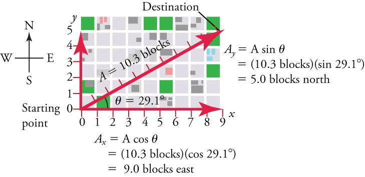
A map is shown over top x and y-axes. The origin is labeled Starting Point. The x-axis represents east and has a scale from zero to nine in increments of one. The y-axis represents north and has a scale from zero to five in increments of one. Lines show that a person walks nine blocks east and five blocks north. A displacement vector is plotted from the origin to the destination of nine, five on the axes. The following label is next to the y-axis: A y equals A times sine angle, equals ten point three bloc

Then A = 10.3 blocks and θ = 29.1 ∘ θ = 29.1 ∘ , so that

This magnitude indicates that the walker has traveled 9 blocks to the east—in other words, a 9-block eastward displacement. Similarly,

indicating that the walker has traveled 5 blocks to the north—a 5-block northward displacement.

Analytical Method of Vector Addition and Subtraction

Calculating a resultant vector (or vector addition) is the reverse of breaking the resultant down into its components. If the perpendicular components A x A x and A y A y of a vector A A are known, then we can find A A analytically. How do we do this? Since, by definition,

we solve for θ θ to find the direction of the resultant.

Since this is a right triangle, the Pythagorean theorem (x 2 + y 2 = h 2 ) for finding the hypotenuse applies. In this case, it becomes

Solving for A gives

In summary, to find the magnitude A A and direction θ θ of a vector from its perpendicular components A x A x and A y A y , as illustrated in Figure 5.22 , we use the following relationships:

Vectors Ax and Ay form the legs of a right triangle and vector A forms the hypotenuse. Vectors Ax and Ay are dashed. The formula angle equals inverse tangent times Ay over Ax is inside the triangle. Vector A is labeled A equals the square root of Ax squared plus Ay squared.

Sometimes, the vectors added are not perfectly perpendicular to one another. An example of this is the case below, where the vectors A A and B B are added to produce the resultant R , R , as illustrated in Figure 5.23 .

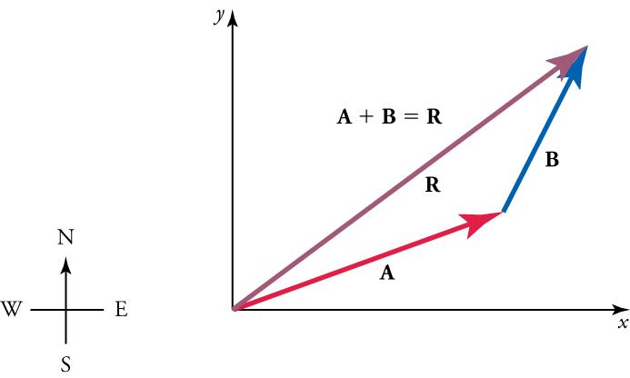
A compass is shown on the left. On the right, vectors A, B, and R form a triangle, with the vertex of AR at the origin of an x-y axis. The formula A plus B equals R is above the triangle.

If A A and B B represent two legs of a walk (two displacements), then R R is the total displacement. The person taking the walk ends up at the tip of R R . There are many ways to arrive at the same point. The person could have walked straight ahead first in the x -direction and then in the y -direction. Those paths are the x - and y -components of the resultant, R x R x and R y . R y . If we know R x R x and R y R y , we can find R R and θ θ using the equations R = R x 2 + R y 2 R = R x 2 + R y 2 and θ = t a n – 1 ( R y / R x ) θ = t a n – 1 ( R y / R x ) .

and find the y component of the resultant (as illustrated in Figure 5.25 ) by adding the y component of the vectors.

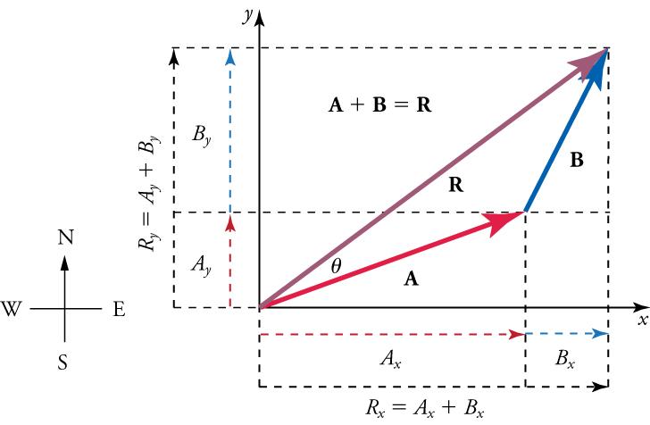
Now that we know the components of R , R , we can find its magnitude and direction.

To get the magnitude of the resultant R, use the Pythagorean theorem. R = R x 2 + R y 2 R = R x 2 + R y 2
To get the direction of the resultant θ = tan − 1 ( R y / R x ) . θ = tan − 1 ( R y / R x ) .

Watch Physics

Classifying vectors and quantities example.

This video contrasts and compares three vectors in terms of their magnitudes, positions, and directions.

0 units . All of them will cancel each other out.
5 units . Two of them will cancel each other out.
10 units . Two of them will add together to give the resultant.
15 units. All of them will add together to give the resultant.

Tips For Success

In the video, the vectors were represented with an arrow above them rather than in bold. This is a common notation in math classes.

Using the Analytical Method of Vector Addition and Subtraction to Solve Problems

Figure 5.26 uses the analytical method to add vectors.

Worked Example

Add the vector A A to the vector B B shown in Figure 5.26 , using the steps above. The x -axis is along the east–west direction, and the y -axis is along the north–south directions. A person first walks 53 .0 m 53 .0 m in a direction 20 .0° 20 .0° north of east, represented by vector A . A . The person then walks 34 .0 m 34 .0 m in a direction 63 .0 ° 63 .0 ° north of east, represented by vector B . B .

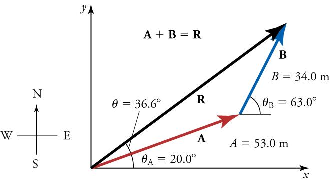
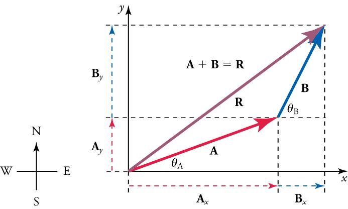
Vectors A, B, and R form a triangle with vertex RA at the origin of an x y-axis. The following labels are included: angle (where R and A form an angle) equals thirty-six point six degrees, angle A equals twenty degrees, angle B equals sixty-three degrees, A equals fifty-three meters, B equals thirty-four meters, and A plus B equals R. A compass is shown in the bottom corner for reference.

The components of A A and B B along the x - and y -axes represent walking due east and due north to get to the same ending point. We will solve for these components and then add them in the x-direction and y-direction to find the resultant.

First, we find the components of A A and B B along the x - and y -axes. From the problem, we know that A = 53.0 m A = 53.0 m , θ A = 20.0 ∘ θ A = 20.0 ∘ , B B = 34 .0 m 34 .0 m , and θ B = 63.0 ∘ θ B = 63.0 ∘ . We find the x -components by using A x = A cos θ A x = A cos θ , which gives

Similarly, the y -components are found using A y = A sin θ A A y = A sin θ A

The x - and y -components of the resultant are

Now we can find the magnitude of the resultant by using the Pythagorean theorem

Finally, we find the direction of the resultant

This example shows vector addition using the analytical method. Vector subtraction using the analytical method is very similar. It is just the addition of a negative vector. That is, A − B ≡ A + ( − B ) A − B ≡ A + ( − B ) . The components of – B B are the negatives of the components of B B . Therefore, the x - and y -components of the resultant A − B = R A − B = R are

and the rest of the method outlined above is identical to that for addition.

Practice Problems

What is the magnitude of a vector whose x -component is 4 cm and whose y -component is 3 cm?

What is the magnitude of a vector that makes an angle of 30° to the horizontal and whose x -component is 3 units?

Links To Physics

Atmospheric science.

A black and white photograph of a meteorologist is shown. The meteorologist is standing in front of a weather map with a television camera pointing at him.

Atmospheric science is a physical science , meaning that it is a science based heavily on physics. Atmospheric science includes meteorology (the study of weather) and climatology (the study of climate). Climate is basically the average weather over a longer time scale. Weather changes quickly over time, whereas the climate changes more gradually.

The movement of air, water and heat is vitally important to climatology and meteorology. Since motion is such a major factor in weather and climate, this field uses vectors for much of its math.

Vectors are used to represent currents in the ocean, wind velocity and forces acting on a parcel of air. You have probably seen a weather map using vectors to show the strength (magnitude) and direction of the wind.

Vectors used in atmospheric science are often three-dimensional. We won’t cover three-dimensional motion in this text, but to go from two-dimensions to three-dimensions, you simply add a third vector component. Three-dimensional motion is represented as a combination of x -, y - and z components, where z is the altitude.

Vector calculus combines vector math with calculus, and is often used to find the rates of change in temperature, pressure or wind speed over time or distance. This is useful information, since atmospheric motion is driven by changes in pressure or temperature. The greater the variation in pressure over a given distance, the stronger the wind to try to correct that imbalance. Cold air tends to be more dense and therefore has higher pressure than warm air. Higher pressure air rushes into a region of lower pressure and gets deflected by the spinning of the Earth, and friction slows the wind at Earth’s surface.

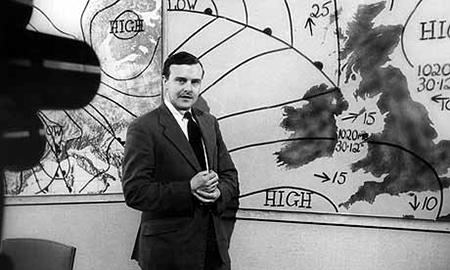
Finding how wind changes over distance and multiplying vectors lets meteorologists, like the one shown in Figure 5.27 , figure out how much rotation (spin) there is in the atmosphere at any given time and location. This is an important tool for tornado prediction. Conditions with greater rotation are more likely to produce tornadoes.

Vectors have magnitude as well as direction and can be quickly solved through scalar algebraic operations.
Vectors have magnitude but no direction, so it becomes easy to express physical quantities involved in the atmospheric science.
Vectors can be solved very accurately through geometry, which helps to make better predictions in atmospheric science.
Vectors have magnitude as well as direction and are used in equations that describe the three dimensional motion of the atmosphere.

Check Your Understanding

Between the analytical and graphical methods of vector additions, which is more accurate? Why?

The analytical method is less accurate than the graphical method, because the former involves geometry and trigonometry.
The analytical method is more accurate than the graphical method, because the latter involves some extensive calculations.
The analytical method is less accurate than the graphical method, because the former includes drawing all figures to the right scale.
The analytical method is more accurate than the graphical method, because the latter is limited by the precision of the drawing.

What is a component of a two dimensional vector?

A component is a piece of a vector that points in either the x or y direction.
A component is a piece of a vector that has half of the magnitude of the original vector.
A component is a piece of a vector that points in the direction opposite to the original vector.
A component is a piece of a vector that points in the same direction as original vector but with double of its magnitude.
θ = cos − 1 ⁡ A y A x
θ = cot − 1 ⁡ A y A x
θ = sin − 1 ⁡ A y A x
θ = tan − 1 ⁡ A y A x

How can we determine the magnitude of a vector if we know the magnitudes of its components?

| A → | = A x + A y | A → | = A x + A y
| A → | = A x 2 + A y 2 | A → | = A x 2 + A y 2
| A → | = ( A x 2 + A y 2 ) 2 | A → | = ( A x 2 + A y 2 ) 2

Copy and paste the link code above.

5.2: Vector Fields

Last updated
Save as PDF
Page ID 64021

Learning Objectives

Recognize a vector field in a plane or in space.
Sketch a vector field from a given equation.
Identify a conservative field and its associated potential function.
Explain how to find a potential function for a conservative vector field.
Explain how to test a vector field to determine whether it is conservative.

Vector fields are an important tool for describing many physical concepts, such as gravitation and electromagnetism, which affect the behavior of objects over a large region of a plane or of space. They are also useful for dealing with large-scale behavior such as atmospheric storms or deep-sea ocean currents. In this section, we examine the basic definitions and graphs of vector fields so we can study them in more detail in the rest of this chapter.

Examples of Vector Fields

How can we model the gravitational force exerted by multiple astronomical objects? How can we model the velocity of water particles on the surface of a river? Figure $\PageIndex{1}$ gives visual representations of such phenomena.

$Two images, labeled A and B. Image A shows the gravitational field exerted by two astronomical bodies on a small object. The earth is on the left, and the moon is on the right. The earth is surrounded by long arrows pointing towards its center arranged in concentric circles. There is a break in the circle on the right, across from the moon. The moon is surrounded by smaller arrows that curve out and to the right. Image B shows the vector velocity field of water on the surface of a river with a large rock in the middle. The arrows tend to point at the same angle as the riverbank. Where the river meets the rock, the arrows point around the rock. After the rock, the some arrows point forward, and others turn back to the rock. The water flows fastest towards the middle of the river and around the rock and slowest along the riverbank.$

Figure $\PageIndex{1a}$ shows a gravitational field exerted by two astronomical objects, such as a star and a planet or a planet and a moon. At any point in the figure, the vector associated with a point gives the net gravitational force exerted by the two objects on an object of unit mass. The vectors of largest magnitude in the figure are the vectors closest to the larger object. The larger object has greater mass, so it exerts a gravitational force of greater magnitude than the smaller object.

Figure $\PageIndex{1b}$ shows the velocity of a river at points on its surface. The vector associated with a given point on the river’s surface gives the velocity of the water at that point. Since the vectors to the left of the figure are small in magnitude, the water is flowing slowly on that part of the surface. As the water moves from left to right, it encounters some rapids around a rock. The speed of the water increases, and a whirlpool occurs in part of the rapids.

Each figure illustrates an example of a vector field. Intuitively, a vector field is a map of vectors. In this section, we study vector fields in $ℝ^2$ and $ℝ^3$.

DEFINITION: vector field

A vector field $\vecs{F}$ in $ℝ^2$ is an assignment of a two-dimensional vector $\vecs{F}(x,y)$ to each point $(x,y)$ of a subset $D$ of $ℝ^2$. The subset $D$ is the domain of the vector field.
A vector field $\vecs{F}$ in $ℝ^3$ is an assignment of a three-dimensional vector $\vecs{F}(x,y,z)$ to each point $(x,y,z)$ of a subset $D$ of $ℝ^3$. The subset $D$ is the domain of the vector field.

Vector Fields in $ℝ^2$

A vector field in $ℝ^2$ can be represented in either of two equivalent ways. The first way is to use a vector with components that are two-variable functions:

\[\vecs{F}(x,y)=⟨P(x,y),Q(x,y)⟩\]

The second way is to use the standard unit vectors:

\[\vecs{F}(x,y)=P(x,y) \,\hat{\mathbf i}+Q(x,y) \,\hat{\mathbf j}.\]

A vector field is said to be continuous if its component functions are continuous.

Example $\PageIndex{1}$: Finding a Vector Associated with a Given Point

Let $\vecs{F} (x,y)=(2y^2+x−4)\,\hat{\mathbf i}+\cos(x)\,\hat{\mathbf j}$ be a vector field in $ℝ^2$. Note that this is an example of a continuous vector field since both component functions are continuous. What vector is associated with point $(0,−1)$?

Substitute the point values for $x$ and $y$:

\[\begin{align*} \vecs{F} (0,-1) &=(2{(−1)}^2+0−4) \,\hat{\mathbf i}+\cos(0) \,\hat{\mathbf j} \\[4pt] &=−2 \,\hat{\mathbf i} + \hat{\mathbf j}. \end{align*}\]

Exercise $\PageIndex{1}$

Let $\vecs{G}(x,y)=x^2y\,\hat{\mathbf i}−(x+y)\,\hat{\mathbf j}$ be a vector field in $ℝ^2$. What vector is associated with the point $(−2,3)$?

Substitute the point values into the vector function.

$\vecs{G}(−2,3)=12\hat{\mathbf i}−\hat{\mathbf j}$

Drawing a Vector Field

We can now represent a vector field in terms of its components of functions or unit vectors, but representing it visually by sketching it is more complex because the domain of a vector field is in $ℝ^2$, as is the range. Therefore the “graph” of a vector field in $ℝ^2$ lives in four-dimensional space. Since we cannot represent four-dimensional space visually, we instead draw vector fields in $ℝ^2$ in a plane itself. To do this, draw the vector associated with a given point at the point in a plane. For example, suppose the vector associated with point $(4,−1)$ is $⟨3,1⟩$. Then, we would draw vector $⟨3,1⟩$ at point $(4,−1)$.

We should plot enough vectors to see the general shape, but not so many that the sketch becomes a jumbled mess. If we were to plot the image vector at each point in the region, it would fill the region completely and is useless. Instead, we can choose points at the intersections of grid lines and plot a sample of several vectors from each quadrant of a rectangular coordinate system in $ℝ^2$.

There are two types of vector fields in $ℝ^2$ on which this chapter focuses: radial fields and rotational fields. Radial fields model certain gravitational fields and energy source fields, and rotational fields model the movement of a fluid in a vortex. In a radial field, all vectors either point directly toward or directly away from the origin. Furthermore, the magnitude of any vector depends only on its distance from the origin. In a radial field, the vector located at point $(x,y)$ is perpendicular to the circle centered at the origin that contains point $(x,y)$, and all other vectors on this circle have the same magnitude.

Example $\PageIndex{2}$: Drawing a Radial Vector Field

Sketch the vector field $\vecs{F} (x,y)=\dfrac{x}{2}\hat{\mathbf i}+\dfrac{y}{2}\hat{\mathbf j}$.

To sketch this vector field, choose a sample of points from each quadrant and compute the corresponding vector. The following table gives a representative sample of points in a plane and the corresponding vectors.

Figure $\PageIndex{2a}$ shows the vector field. To see that each vector is perpendicular to the corresponding circle, Figure $\PageIndex{2b}$ shows circles overlain on the vector field.

$A visual representation of the given vector field in a coordinate plane with two additional diagrams with notation. The first representation shows the vector field. The arrows are circling the origin in a clockwise motion. The second representation shows concentric circles, highlighting the radial pattern. The The third representation shows the concentric circles. It also shows arrows for the radial vector <a,b> for all points (a,b). Each is perpendicular to the arrows in the given vector field.$

Exercise $\PageIndex{2}$

Draw the radial field $\vecs{F} (x,y)=−\dfrac{x}{3}\hat{\mathbf i}−\dfrac{y}{3}\hat{\mathbf j}$.

Sketch enough vectors to get an idea of the shape.

$A visual representation of the given radial field in a coordinate plane. The magnitudes increase further from the origin. The arrow seem to be stretching away from the origin in a rectangular shape.$

In contrast to radial fields, in a rotational field , the vector at point $(x,y)$ is tangent (not perpendicular) to a circle with radius $r=\sqrt{x^2+y^2}$. In a standard rotational field, all vectors point either in a clockwise direction or in a counterclockwise direction, and the magnitude of a vector depends only on its distance from the origin. Both of the following examples are clockwise rotational fields, and we see from their visual representations that the vectors appear to rotate around the origin.

Example $\PageIndex{3}$: Drawing a Rotational Vector Field

Sketch the vector field $\vecs{F} (x,y)=⟨y,\,−x⟩$.

Create a table (see the one that follows) using a representative sample of points in a plane and their corresponding vectors. Figure $\PageIndex{3}$ shows the resulting vector field.

$clipboard_eefd79a8783ad793483370902770aaa4f.png$

Note that vector $\vecs{F}(a,b)=⟨b,−a⟩$ points clockwise and is perpendicular to radial vector $⟨a,b⟩$. (We can verify this assertion by computing the dot product of the two vectors: $⟨a,b⟩·⟨−b,a⟩=−ab+ab=0$.) Furthermore, vector $⟨b,−a⟩$ has length $r=\sqrt{a^2+b^2}$. Thus, we have a complete description of this rotational vector field: the vector associated with point $(a,b)$ is the vector with length r tangent to the circle with radius r , and it points in the clockwise direction.

Sketches such as that in Figure $\PageIndex{3}$ are often used to analyze major storm systems, including hurricanes and cyclones. In the northern hemisphere, storms rotate counterclockwise; in the southern hemisphere, storms rotate clockwise. (This is an effect caused by Earth’s rotation about its axis and is called the Coriolis Effect .)

$A photgraph of a hurricane, showing the rotation around its eye.$

Example $\PageIndex{4}$: Sketching a Vector Field

Sketch vector field $\vecs{F}(x,y)=\dfrac{y}{x^2+y^2}\hat{\mathbf i}, -\dfrac{x}{x^2+y^2}\hat{\mathbf j}$.

To visualize this vector field, first note that the dot product $\vecs{F}(a,b)·(a \,\hat{\mathbf i}+b \,\hat{\mathbf j})$ is zero for any point $(a,b)$. Therefore, each vector is tangent to the circle on which it is located. Also, as $(a,b)\rightarrow(0,0)$, the magnitude of $\vecs{F}(a,b)$ goes to infinity. To see this, note that

$||\vecs{F}(a,b)||=\sqrt{\dfrac{a^2+b^2}{ {(a^2+b^2)}^2 }} =\sqrt{\dfrac{1}{a^2+b^2}}$.

Since $\dfrac{1}{a^2+b^2}\rightarrow \infty$ as $(a,b)\rightarrow (0,0)$, then $||\vecs F(a,b)||\rightarrow \infty$ as $(a,b)\rightarrow (0,0)$. This vector field looks similar to the vector field in Example $\PageIndex{3}$, but in this case the magnitudes of the vectors close to the origin are large. Table $\PageIndex{3}$ shows a sample of points and the corresponding vectors, and Figure $\PageIndex{5}$ shows the vector field. Note that this vector field models the whirlpool motion of the river in Figure $\PageIndex{5}$(b). The domain of this vector field is all of $ℝ^2$ except for point $(0,0)$.

$A visual representation of the given vector field in a coordinate plane. The magnitude is larger closer to the origin. The arrows are rotating the origin clockwise. It could be use to model whirlpool motion of a fluid.$

Exercise $\PageIndex{4}$

Sketch vector field $\vecs{F}(x,y)=⟨−2y,\,2x⟩$. Is the vector field radial, rotational, or neither?

Substitute enough points into $\vecs{F}$ to get an idea of the shape.

$A visual representation of a rotational vector field in a coordinate plane. The arrows circle the origin in a counterclockwise manner.$

Example $\PageIndex{5}$: Velocity Field of a Fluid

Suppose that $\vecs{v} (x,y)=−\dfrac{2y}{x^2+y^2}\hat{\mathbf i}+\dfrac{2x}{x^2+y^2}\hat{\mathbf j}$ is the velocity field of a fluid. How fast is the fluid moving at point $(1,−1)$? (Assume the units of speed are meters per second.)

To find the velocity of the fluid at point $(1,−1)$, substitute the point into $\vecs{v} $:

$\vecs{v}(1,−1)=\dfrac{−2(−1)}{1+1}\hat{\mathbf i}+\dfrac{2(1)}{1+1}\hat{\mathbf j}=\hat{\mathbf i}+\hat{\mathbf j}$.

The speed of the fluid at $(1,−1)$ is the magnitude of this vector. Therefore, the speed is $||\hat{\mathbf i}+\hat{\mathbf j}||=\sqrt{2}$ m/sec.

Exercise $\PageIndex{5}$

Vector field $\vecs{v} (x,y)=⟨4|x|,\,1⟩$ models the velocity of water on the surface of a river. What is the speed of the water at point $(2,3)$? Use meters per second as the units.

Remember, speed is the magnitude of velocity.

$\sqrt{65}$ m/sec

We have examined vector fields that contain vectors of various magnitudes, but just as we have unit vectors, we can also have a unit vector field. A vector field $\vecs{F}$ is a unit vector field if the magnitude of each vector in the field is 1. In a unit vector field, the only relevant information is the direction of each vector.

Example $\PageIndex{6}$: A Unit Vector Field

Show that vector field $\vecs{F} (x,y)=\left\langle\dfrac{y}{\sqrt{x^2+y^2}},−\dfrac{x}{\sqrt{x^2+y^2}}\right\rangle$ is a unit vector field.

To show that $\vecs{F}$ is a unit field, we must show that the magnitude of each vector is $1$. Note that

\[\begin{align*} \sqrt{ \left(\dfrac{y}{\sqrt{x^2+y^2}}\right)^2+\left(−\dfrac{x}{\sqrt{x^2+y^2}}\right)^2} &=\sqrt{ \dfrac{y^2}{x^2+y^2}+\dfrac{x^2}{x^2+y^2}} \\[4pt] &=\sqrt{\dfrac{x^2+y^2}{x^2+y^2}} \\[4pt] &=1 \end{align*}\]

Therefore, $\vecs{F} $ is a unit vector field.

Exercise $\PageIndex{6}$

Is vector field $\vecs{F} (x,y)=⟨−y,\,x⟩$ a unit vector field?

Calculate the magnitude of $\vecs{F} $ at an arbitrary point $(x,y)$.

Why are unit vector fields important? Suppose we are studying the flow of a fluid, and we care only about the direction in which the fluid is flowing at a given point. In this case, the speed of the fluid (which is the magnitude of the corresponding velocity vector) is irrelevant, because all we care about is the direction of each vector. Therefore, the unit vector field associated with velocity is the field we would study.

If $\vecs{F} =⟨P,Q,R⟩$ is a vector field, then the corresponding unit vector field is $\big\langle\tfrac{P}{||\vecs F||},\tfrac{Q}{||\vecs F||},\tfrac{R}{||\vecs F||}\big\rangle$. Notice that if $\vecs{F}(x,y)=⟨y,\,−x⟩$ is the vector field from Example $\PageIndex{6}$, then the magnitude of $\vecs{F} $ is $\sqrt{x^2+y^2}$, and therefore the corresponding unit vector field is the field $\vecs{G} $ from the previous example.

If $\vecs{F} $ is a vector field, then the process of dividing $\vecs{F} $ by its magnitude to form unit vector field $\vecs{F}/||\vecs{F}||$ is called normalizing the field $\vecs{F} $.

Vector Fields in $ℝ^3$

We have seen several examples of vector fields in $ℝ^2$; let’s now turn our attention to vector fields in $ℝ^3$. These vector fields can be used to model gravitational or electromagnetic fields, and they can also be used to model fluid flow or heat flow in three dimensions. A two-dimensional vector field can really only model the movement of water on a two-dimensional slice of a river (such as the river’s surface). Since a river flows through three spatial dimensions, to model the flow of the entire depth of the river, we need a vector field in three dimensions.

The extra dimension of a three-dimensional field can make vector fields in $ℝ^3$ more difficult to visualize, but the idea is the same. To visualize a vector field in $ℝ^3$, plot enough vectors to show the overall shape. We can use a similar method to visualizing a vector field in $ℝ^2$ by choosing points in each octant.

Just as with vector fields in $ℝ^2$, we can represent vector fields in $ℝ^3$ with component functions. We simply need an extra component function for the extra dimension. We write either

\[\vecs{F}(x,y,z)=⟨P(x,y,z),Q(x,y,z),R(x,y,z)⟩\]

\[\vecs{F}(x,y,z)=P(x,y,z)\hat{\mathbf i}+Q(x,y,z)\hat{\mathbf j}+R(x,y,z)\hat{\mathbf k}.\]

Example $\PageIndex{7}$: Sketching a Vector Field in Three Dimensions

Describe vector field $\vecs{F}(x,y,z)=⟨1,\,1,\,z⟩$.

For this vector field, the $x$- and $y$-components are constant, so every point in $ℝ^3$ has an associated vector with $x$- and $y$-components equal to one. To visualize $\vecs{F}$, we first consider what the field looks like in the $xy$-plane. In the $xy$-plane, $z=0$. Hence, each point of the form $(a,b,0)$ has vector $⟨1,1,0⟩$ associated with it. For points not in the $xy$-plane but slightly above it, the associated vector has a small but positive $z$-component, and therefore the associated vector points slightly upward. For points that are far above the $xy$-plane, the $z$-component is large, so the vector is almost vertical. Figure $\PageIndex{6}$ shows this vector field.

Figure $\PageIndex{6}$: A visual representation of vector field $\vecs{F}(x,y,z)=⟨1,1,z⟩$.

Exercise $\PageIndex{7}$

Sketch vector field $\vecs{G}(x,y,z)=⟨2,\,\dfrac{z}{2},\,1⟩$.

Substitute enough points into the vector field to get an idea of the general shape.

In the next example, we explore one of the classic cases of a three-dimensional vector field: a gravitational field.

Example $\PageIndex{8}$: Describing a Gravitational Vector Field

Newton’s law of gravitation states that $\vecs{F}=−G\dfrac{m_1m_2}{r^2}\hat{\mathbf r}$, where G is the universal gravitational constant. It describes the gravitational field exerted by an object (object 1) of mass $m_1$ located at the origin on another object (object 2) of mass $m_2$ located at point $(x,y,z)$. Field $\vecs{F}$ denotes the gravitational force that object 1 exerts on object 2, $r$ is the distance between the two objects, and $\hat{\mathbf r}$ indicates the unit vector from the first object to the second. The minus sign shows that the gravitational force attracts toward the origin; that is, the force of object 1 is attractive. Sketch the vector field associated with this equation.

Since object 1 is located at the origin, the distance between the objects is given by $r=\sqrt{x^2+y^2+z^2}$. The unit vector from object 1 to object 2 is $\hat{\mathbf r}=\dfrac{⟨x,y,z⟩}{||⟨x,y,z⟩||}$, and hence $\hat{\mathbf r}=\big\langle\dfrac{x}{r},\dfrac{y}{r},\dfrac{z}{r}\big\rangle$. Therefore, gravitational vector field $\vecs{F}$ exerted by object 1 on object 2 is

\[ \vecs{F}=−Gm_1m_2\big\langle\dfrac{x}{r^3},\dfrac{y}{r^3},\dfrac{z}{r^3}\big\rangle. \nonumber\]

This is an example of a radial vector field in $ℝ^3$.

Figure $\PageIndex{7}$ shows what this gravitational field looks like for a large mass at the origin. Note that the magnitudes of the vectors increase as the vectors get closer to the origin.

$A visual representation of the given gravitational vector field in three dimensions. The magnitudes of the vectors increase as the vectors get closer to the origin. The arrows point in, towards the mass at the origin.$

Exercise $\PageIndex{8}$

The mass of asteroid 1 is 750,000 kg and the mass of asteroid 2 is 130,000 kg. Assume asteroid 1 is located at the origin, and asteroid 2 is located at $(15,−5,10)$, measured in units of 10 to the eighth power kilometers. Given that the universal gravitational constant is $G=6.67384×10^{−11}m^3{kg}^{−1}s^{−2}$, find the gravitational force vector that asteroid 1 exerts on asteroid 2.

Follow Example $\PageIndex{8}$ and first compute the distance between the asteroids.

$1.49063×{10}^{−18}$, $4.96876×{10}^{−19}$, $9.93752×{10}^{−19}$ N

Gradient Fields (Conservative Fields)

In this section, we study a special kind of vector field called a gradient field or a conservative field . These vector fields are extremely important in physics because they can be used to model physical systems in which energy is conserved. Gravitational fields and electric fields associated with a static charge are examples of gradient fields.

Recall that if $f$ is a (scalar) function of $x$ and $y$, then the gradient of $f$ is

\[ \text{grad}\, f =\vecs \nabla f(x,y) =f_x(x,y) \hat{\mathbf i} +f_y(x,y) \hat{\mathbf j}. \]

We can see from the form in which the gradient is written that $\vecs \nabla f$ is a vector field in $ℝ^2$. Similarly, if $f$ is a function of $x$, $y$, and $z$, then the gradient of $f$ is

\[ \text{grad}\, f =\vecs \nabla f(x,y,z) = f_x(x,y,z) \hat{\mathbf i}+f_y(x,y,z) \hat{\mathbf j}+f_z(x,y,z)\hat{\mathbf k}. \]

The gradient of a three-variable function is a vector field in $ℝ^3$. A gradient field is a vector field that can be written as the gradient of a function, and we have the following definition.

DEFINITION: Gradient Field

A vector field $\vecs{F}$ in $ℝ^2$ or in $ℝ^3$ is a gradient field if there exists a scalar function $f$ such that $\vecs \nabla f=\vecs{F}$.

Example $\PageIndex{9}$: Sketching a Gradient Vector Field

Use technology to plot the gradient vector field of $f(x,y)=x^2y^2$.

The gradient of $f$ is $\vecs \nabla f(x,y)=⟨2xy^2,\,2x^2y⟩$. To sketch the vector field, use a computer algebra system such as Mathematica. Figure $\PageIndex{8}$ shows $\vecs \nabla f$.

$A visual representation of the given gradient vector field in two dimensions. The arrows point up above the x axis and down below the x axis, and they point left on the left side of the y axis and to the right on the right side of the y axis. The further the arrows are from zero, the more vertical they are, and the closer the arrows are to zero, the more horizontal they are.$

Exercise $\PageIndex{9}$

Use technology to plot the gradient vector field of $f(x,y)=\sin x\cos y$.

Find the gradient of $f$.

$A visual representation of the given given vector in two dimensions. The arrows seem to be forming several ovals. The first is around the origin, where the arrows curve to the right above and below the x axis. The closer the arrows are to the x axis, the flatter they are. There appear to be six other ovals, three on either side of the central one. The vectors get longer as they get farther from the origin, and then they start to get shorter again.$

Consider the function $f(x,y)=x^2y^2$ from Example $\PageIndex{9}$. Figure $\PageIndex{9}$ shows the level curves of this function overlaid on the function’s gradient vector field. The gradient vectors are perpendicular to the level curves, and the magnitudes of the vectors get larger as the level curves get closer together, because closely grouped level curves indicate the graph is steep, and the magnitude of the gradient vector is the largest value of the directional derivative. Therefore, you can see the local steepness of a graph by investigating the corresponding function’s gradient field.

$A visual representation of the given gradient field. The arrows are flatter the closer they are to the x axis and more vertical the further they are from the x axis. The arrows point left to the left of the y axis, and they point to the right to the right of the y axis. They point up above the x axis and down below the x axis. Severl level curves are drawn, each asymptotically approaching the axes. As the level curves get closer together, the magnitude of the gradient vactors increases.$

As we learned earlier, a vector field $\vecs{F}$ is a conservative vector field, or a gradient field if there exists a scalar function $f$ such that $\vecs \nabla f=\vecs{F}$. In this situation, $f$ is called a potential function for $\vecs{F}$. Conservative vector fields arise in many applications, particularly in physics. The reason such fields are called conservative is that they model forces of physical systems in which energy is conserved. We study conservative vector fields in more detail later in this chapter.

You might notice that, in some applications, a potential function $f$ for $\vecs{F}$ is defined instead as a function such that $−\vecs \nabla f=\vecs{F}$. This is the case for certain contexts in physics, for example.

Example $\PageIndex{10}$: Verifying a Potential Function

Is $f(x,y,z)=x^2yz−\sin(xy)$ a potential function for vector field

$\vecs{F}(x,y,z)=⟨2xyz−y\cos(xy),x^2z−x\cos(xy),x^2y⟩$?

We need to confirm whether $\vecs \nabla f=\vecs{F}$. We have

\[ \begin{align*} f_x(x,y) =2xyz−y\cos(xy) \\[4pt] f_y(x,y) =x^2z−x\cos(xy) \\[4pt] f_z(x,y) =x^2y \end{align*}.\]

Therefore, $\vecs \nabla f=\vecs{F}$ and $f$ is a potential function for $\vecs{F}$.

Exercise $\PageIndex{10}$

Is $f(x,y,z)=x^2\cos(yz)+y^2z^2$ a potential function for $\vecs{F}(x,y,z)=⟨2x\cos(yz),−x^2z \sin(yz)+2yz^2,y^2⟩$?

Compute the gradient of $f$.

Example $\PageIndex{11}$: Verifying a Potential Function

The velocity of a fluid is modeled by field $\vecs v(x,y)=⟨xy,\tfrac{x^2}{2}−y⟩$. Verify that $f(x,y)=\dfrac{x^2y}{2}−\dfrac{y^2}{2}$ is a potential function for $\vecs{v}$.

To show that $f$ is a potential function, we must show that $\vecs \nabla f=\vecs v$. Note that $f_x(x,y)=xy$ and $f_y(x,y)=\dfrac{x^2}{2}−y$. Therefore, $\vecs \nabla f(x,y)=⟨xy,\tfrac{x^2}{2}−y⟩$ and $f$ is a potential function for $\vecs{v}$ (Figure $\PageIndex{10}$).

$A visual representation of the given directional field in two dimensions. The arrows in quadrant 1point to the right. Closer to the y axis, they point down, but they quickly cuve and soon point up at at roughly 90-degree angle. The closer the arrows are to the x axis, the more vertical they are. Quadrant 2 is a reflection of quadrant 1. In quadrant 3, the arrows are more vertical the closer they are to the x and y axes. They point up and to the right. The further they are from the axes, the closer the arrows are to a 90-degree angle. Quadrant 4 is a reflection of quadrant 3.$

Exercise $\PageIndex{11}$

Verify that $f(x,y)=x^2y^2+x$ is a potential function for velocity field $\vecs{v}(x,y)=⟨3x^2y^2+1,2x^3y⟩$.

Calculate the gradient.

$\vecs \nabla f(x,y)=\vecs{v}(x,y)$

If $\vecs{F}$ is a conservative vector field, then there is at least one potential function $f$ such that $\vecs \nabla f=\vecs{F}$. But, could there be more than one potential function? If so, is there any relationship between two potential functions for the same vector field? Before answering these questions, let’s recall some facts from single-variable calculus to guide our intuition. Recall that if $k(x)$ is an integrable function, then $k$ has infinitely many antiderivatives. Furthermore, if $\vecs{F}$ and $\vecs{G}$ are both antiderivatives of $k$, then $\vecs{F}$ and $\vecs{G}$ differ only by a constant . That is, there is some number $C$ such that $\vecs{F}(x)=\vecs{G}(x)+C$.

Now let $\vecs{F}$ be a conservative vector field and let $f$ and $g$ be potential functions for $\vecs{F}$. Since the gradient is like a derivative, $\vecs{F}$ being conservative means that $\vecs{F}$ is “integrable” with “antiderivatives” $f$ and $g$. Therefore, if the analogy with single-variable calculus is valid, we expect there is some constant $C$ such that $f(x)=g(x)+C$. The next theorem says that this is indeed the case.

To state the next theorem with precision, we need to assume the domain of the vector field is connected and open. To be connected means if $P_1$ and $P_2$ are any two points in the domain, then you can walk from $P_1$ to $P_2$ along a path that stays entirely inside the domain.

UNIQUENESS OF POTENTIAL FUNCTIONS

Let $\vecs{F}$ be a conservative vector field on an open and connected domain and let $f$ and $g$ be functions such that $\vecs \nabla f=\vecs{F}$ and $\vecs \nabla g=\vecs{G}$. Then, there is a constant $C$ such that $f=g+C$.

Since $f$ and $g$ are both potential functions for $\vecs{F}$, then $\vecs \nabla (f−g)=\vecs \nabla f−\vecs \nabla g=\vecs{F}−\vecs{F}=\vecs 0$. Let $h=f−g$, then we have $\vecs \nabla h=\vecs 0$.We would like to show that $h$ is a constant function.

Assume $h$ is a function of $x$ and $y$ (the logic of this proof extends to any number of independent variables). Since $\vecs \nabla h=\vecs 0$, we have $h_x(x,y)=0$ and $h_y(x,y)=0$. The expression $h_x(x,y)=0$ implies that $h$ is a constant function with respect to $x$—that is, $h(x,y)=k_1(y)$ for some function $k_1$. Similarly, $h_y(x,y)=0$ implies $h(x,y)=k_2(x)$ for some function $k_2$. Therefore, function $h$ depends only on $y$ and also depends only on $x$. Thus, $h(x,y)=C$ for some constant $C$ on the connected domain of $\vecs{F}$. Note that we really do need connectedness at this point; if the domain of $\vecs{F}$ came in two separate pieces, then $k$ could be a constant $C_1$ on one piece but could be a different constant $C_2$ on the other piece. Since $f−g=h=C$, we have that $f=g+C$, as desired.

$\square$

Conservative Vector Fields and Potential Functions

As we have learned, the Fundamental Theorem for Line Integrals says that if $\vecs{F}$ is conservative, then calculating $\int_C \vecs F·d\vecs r$ has two steps: first, find a potential function $f$ for $\vecs{F}$ and, second, calculate $f(P_1)−f(P_0)$, where $P_1$ is the endpoint of $C$ and $P_0$ is the starting point. To use this theorem for a conservative field $\vecs{F}$, we must be able to find a potential function $f$ for $\vecs{F}$. Therefore, we must answer the following question: Given a conservative vector field $\vecs{F}$, how do we find a function $f$ such that $\vecs \nabla f=\vecs{F}$? Before giving a general method for finding a potential function, let’s motivate the method with an example.

Example $\PageIndex{5}$: Finding a Potential Function

Find a potential function for $\vecs F(x,y)=⟨2xy^3,3x^2y^2+\cos(y)⟩$, thereby showing that $\vecs{F}$ is conservative.

Suppose that $f(x,y)$ is a potential function for $\vecs{F}$. Then, $\vecs \nabla f=\vecs F$, and therefore

\[f_x(x,y)=2xy^3 \; \; \text{and} \;\; f_y(x,y)=3x^2y^2+\cos y. \nonumber\]

Integrating the equation $f_x(x,y)=2xy^3$ with respect to $x$ yields the equation

\[f(x,y)=x^2y^3+h(y). \nonumber\]

Notice that since we are integrating a two-variable function with respect to $x$, we must add a constant of integration that is a constant with respect to $x$, but may still be a function of $y$. The equation $f(x,y)=x^2y^3+h(y)$ can be confirmed by taking the partial derivative with respect to $x$:

\[\dfrac{∂f}{∂x}=\dfrac{∂}{∂x}(x^2y^3)+\dfrac{∂}{∂x}(h(y))=2xy^3+0=2xy^3. \nonumber\]

Since $f$ is a potential function for $\vecs{F}$,

\[f_y(x,y)=3x^2y^2+\cos(y), \nonumber\]

and therefore

\[3x^2y^2+g′(y)=3x^2y^2+\cos(y). \nonumber\]

This implies that $h′(y)=\cos y$, so $h(y)=\sin y+C$. Therefore, any function of the form $f(x,y)=x^2y^3+\sin(y)+C$ is a potential function. Taking, in particular, $C=0$ gives the potential function $f(x,y)=x^2y^3+\sin(y)$.

To verify that $f$ is a potential function, note that $\vecs \nabla f(x,y)=⟨2xy^3,3x^2y^2+\cos y⟩=\vecs F$.

Find a potential function for $\vecs{F}(x,y)=⟨e^xy^3+y,3e^xy^2+x⟩$.

Follow the steps in Example $\PageIndex{5}$.

$f(x,y)=e^xy^3+xy$

The logic of the previous example extends to finding the potential function for any conservative vector field in $ℝ^2$. Thus, we have the following problem-solving strategy for finding potential functions:

PROBLEM-SOLVING STRATEGY: FINDING A POTENTIAL FUNCTION FOR A CONSERVATIVE VECTOR FIELD $\vecs{F}(x,y)=⟨P(x,y),Q(x,y)⟩$

Integrate $P$ with respect to $x$. This results in a function of the form $g(x,y)+h(y)$, where $h(y)$ is unknown.
Take the partial derivative of $g(x,y)+h(y)$ with respect to $y$, which results in the function $gy(x,y)+h′(y)$.
Use the equation $gy(x,y)+h′(y)=Q(x,y)$ to find $h′(y)$.
Integrate $h′(y)$ to find $h(y)$.
Any function of the form $f(x,y)=g(x,y)+h(y)+C$, where $C$ is a constant, is a potential function for $\vecs{F}$.

We can adapt this strategy to find potential functions for vector fields in $ℝ^3$, as shown in the next example.

Example $\PageIndex{6}$: Finding a Potential Function in $ℝ^3$

Find a potential function for $F(x,y,z)=⟨2xy,x^2+2yz^3,3y^2z^2+2z⟩$, thereby showing that $\vecs{F}$ is conservative.

Suppose that $f$ is a potential function. Then, $\vecs \nabla f= \vecs{F}$ and therefore $f_x(x,y,z)=2xy$. Integrating this equation with respect to $x$ yields the equation $f(x,y,z)=x^2y+g(y,z)$ for some function $g$. Notice that, in this case, the constant of integration with respect to $x$ is a function of $y$ and $z$.

Since $f$ is a potential function,

\[x^2+2yz^3=f_y(x,y,z)=x^2+g_y(y,z). \nonumber\]

\[g_y(y,z)=2yz^3. \nonumber\]

Integrating this function with respect to $y$ yields

\[g(y,z)=y^2z^3+h(z) \nonumber\]

for some function $h(z)$ of $z$ alone. (Notice that, because we know that $g$ is a function of only $y$ and $z$, we do not need to write $g(y,z)=y^2z^3+h(x,z)$.) Therefore,

\[f(x,y,z)=x^2y+g(y,z)=x^2y+y^2z^3+h(z). \nonumber\]

To find $f$, we now must only find $h$. Since $f$ is a potential function,

\[3y^2z^2+2z=g_z(y,z)=3y^2z^2+h′(z). \nonumber\]

This implies that $h′(z)=2z$, so $h(z)=z^2+C$. Letting $C=0$ gives the potential function

\[f(x,y,z)=x^2y+y^2z^3+z^2. \nonumber\]

To verify that $f$ is a potential function, note that $\vecs \nabla f(x,y,z)=⟨2xy,x^2+2yz^3,3y^2z^2+2z⟩=\vecs F(x,y,z)$.

Find a potential function for $\vecs{F}(x,y,z)=⟨12x^2,\cos y\cos z,1−\sin y\sin z⟩$.

Following Example $\PageIndex{6}$, begin by integrating with respect to $x$ .

$f(x,y,z)=4x^3+\sin y\cos z+z$

We can apply the process of finding a potential function to a gravitational force. Recall that, if an object has unit mass and is located at the origin, then the gravitational force in $ℝ^2$ that the object exerts on another object of unit mass at the point $(x,y)$ is given by vector field

$\vecs F(x,y)=−G\left\langle\dfrac{x}{ {(x^2+y^2)}^{3/2} },\dfrac{y}{ {(x^2+y^2)}^{3/2} }\right\rangle$,

where $G$ is the universal gravitational constant. In the next example, we build a potential function for $\vecs{F}$, thus confirming what we already know: that gravity is conservative.

Example $\PageIndex{7}$: Finding a Potential Function

Find a potential function $f$ for $\vecs{F}(x,y)=−G\left\langle\dfrac{x}{ {(x^2+y^2)}^{3/2} },\dfrac{y}{ {(x^2+y^2)}^{3/2} }\right\rangle$.

Suppose that $f$ is a potential function. Then, $\vecs \nabla f= \vecs{F}$ and therefore

\[f_x(x,y)=\dfrac{−Gx}{ {(x^2+y^2)}^{3/2} }.\nonumber\]

To integrate this function with respect to $x$ , we can use $u$-substitution. If $u=x^2+y^2$, then $\dfrac{du}{2}=x\,dx$, so

\[\begin{align*} \int \dfrac{−Gx}{ {(x^2+y^2)}^{3/2} }\,dx &=\int \dfrac{−G}{2u^{3/2}} \,du \\[4pt] &=\dfrac{G}{\sqrt{u}}+h(y) \\[4pt] &=\dfrac{G}{\sqrt{x^2+y^2}}+h(y) \end{align*}\]

for some function $h(y)$. Therefore,

\[f(x,y)=\dfrac{G}{ \sqrt{x^2+y^2}}+h(y).\nonumber\]

\[f_y(x,y)=\dfrac{−Gy}{ {(x^2+y^2)}^{3/2} }\nonumber\].

Since $f(x,y)=\dfrac{G}{ \sqrt{x^2+y^2}}+h(y)$, $f_y(x,y)$ also equals $\dfrac{−Gy}{ {(x^2+y^2)}^{3/2} }+h′(y)$.

\[\dfrac{−Gy}{ {(x^2+y^2)}^{3/2} }+h′(y)=\dfrac{−Gy}{ {(x^2+y^2)}^{3/2} }, \nonumber\]

which implies that $h′(y)=0$. Thus, we can take $h(y)$ to be any constant; in particular, we can let $h(y)=0$. The function

\[f(x,y)=\dfrac{G}{ \sqrt{x^2+y^2} } \nonumber\]

is a potential function for the gravitational field $\vecs{F}$. To confirm that $f$ is a potential function, note that

\[\begin{align*} \vecs\nabla f(x,y) &=⟨−\dfrac{1}{2} \dfrac{G}{ {(x^2+y^2)}^{3/2} } (2x),−\dfrac{1}{2} \dfrac{G}{ {(x^2+y^2)}^{3/2} }(2y)⟩ \\[4pt] &=⟨\dfrac{−Gx}{ {(x^2+y^2)}^{3/2} },\dfrac{−Gy}{ {(x^2+y^2)}^{3/2} }⟩\\[4pt] &=\vecs F(x,y). \end{align*}\]

Find a potential function $f$ for the three-dimensional gravitational force $\vecs{F}(x,y,z)=\left\langle\dfrac{−Gx}{ {(x^2+y^2+z^2)}^{3/2} },\dfrac{−Gy}{ {(x^2+y^2+z^2)}^{3/2} },\dfrac{−Gz}{ {(x^2+y^2+z^2)}^{3/2} }\right\rangle$.

Follow the Problem-Solving Strategy.

$f(x,y,z)=\dfrac{G}{\sqrt{x^2+y^2+z^2}}$

Testing a Vector Field

Until now, we have worked with vector fields that we know are conservative, but if we are not told that a vector field is conservative, we need to be able to test whether it is conservative. Recall that, if $\vecs{F}$ is conservative, then $\vecs{F}$ has the cross-partial property (see The Cross-Partial Property of Conservative Vector Fields). That is, if $\vecs F=⟨P,Q,R⟩$ is conservative, then $P_y=Q_x$, $P_z=R_x$, and $Q_z=R_y$. So, if $\vecs{F}$ has the cross-partial property, then is $\vecs{F}$ conservative? If the domain of $\vecs{F}$ is open and simply connected, then the answer is yes.

Theorem: THE CROSS-PARTIAL TEST FOR CONSERVATIVE FIELDS

If $\vecs{F}=⟨P,Q,R⟩$ is a vector field on an open, simply connected region $D$ and $P_y=Q_x$, $P_z=R_x$, and $Q_z=R_y$ throughout $D$, then $\vecs{F}$ is conservative.

Although a proof of this theorem is beyond the scope of the text, we can discover its power with some examples. Later, we see why it is necessary for the region to be simply connected.

Combining this theorem with the cross-partial property, we can determine whether a given vector field is conservative:

Theorem: CROSS-PARTIAL PROPERTY OF CONSERVATIVE FIELDS

Let $\vecs{F}=⟨P,Q,R⟩$ be a vector field on an open, simply connected region $D$ . Then $P_y=Q_x$, $P_z=R_x$, and $Q_z=R_y$ throughout $D$ if and only if $\vecs{F}$ is conservative.

The version of this theorem in $ℝ^2$ is also true. If $\vecs F(x,y)=⟨P,Q⟩$ is a vector field on an open, simply connected domain in $ℝ^2$, then $\vecs F$ is conservative if and only if $P_y=Q_x$.

Example $\PageIndex{8}$: Determining Whether a Vector Field Is Conservative

Determine whether vector field $\vecs F(x,y,z)=⟨xy^2z,x^2yz,z^2⟩$ is conservative.

Note that the domain of $\vecs{F}$ is all of $ℝ^2$ and $ℝ^3$ is simply connected. Therefore, we can use The Cross-Partial Property of Conservative Vector Fields to determine whether $\vecs{F}$ is conservative. Let

\[P(x,y,z)=xy^2z \nonumber\]

\[Q(x,y,z)=x^2yz \nonumber\]

\[R(x,y,z)=z^2.\nonumber\]

Since $Q_z(x,y,z)=x^2y$ and $R_y(x,y,z)=0$, the vector field is not conservative.

Example $\PageIndex{9}$: Determining Whether a Vector Field Is Conservative

Determine vector field $\vecs{F}(x,y)=⟨x\ln (y), \,\dfrac{x^2}{2y}⟩$ is conservative.

Note that the domain of $\vecs{F}$ is the part of $ℝ^2$ in which $y>0$. Thus, the domain of $\vecs{F}$ is part of a plane above the $x$-axis, and this domain is simply connected (there are no holes in this region and this region is connected). Therefore, we can use The Cross-Partial Property of Conservative Vector Fields to determine whether $\vecs{F}$ is conservative. Let

\[P(x,y)=x\ln (y) \;\; \text{and} \;\;\ Q(x,y)=\dfrac{x^2}{2y}. \nonumber\]

Then $P_y(x,y)=\dfrac{x}{y}=Q_x(x,y)$ and thus $\vecs{F}$ is conservative.

Determine whether $\vecs{F}(x,y)=⟨\sin x\cos y,\,\cos x\sin y⟩$ is conservative.

Use The Cross-Partial Property of Conservative Vector Fields from the previous section.

It is conservative.

When using The Cross-Partial Property of Conservative Vector Fields , it is important to remember that a theorem is a tool, and like any tool, it can be applied only under the right conditions. In the case of The Cross-Partial Property of Conservative Vector Fields , the theorem can be applied only if the domain of the vector field is simply connected.

To see what can go wrong when misapplying the theorem, consider the vector field from Example $\PageIndex{4}$:

\[\vecs F(x,y)=\dfrac{y}{x^2+y^2}\,\hat{\mathbf i}+\dfrac{−x}{x^2+y^2}\,\hat{\mathbf j}.\]

This vector field satisfies the cross-partial property, since

\[\dfrac{∂}{∂y}\left(\dfrac{y}{x^2+y^2}\right)=\dfrac{(x^2+y^2)−y(2y)}{ {(x^2+y^2)}^2}=\dfrac{x^2−y^2}{ {(x^2+y^2)}^2}\]

\[\dfrac{∂}{∂x}\left(\dfrac{−x}{x^2+y^2}\right)=\dfrac{−(x^2+y^2)+x(2x)}{ {(x^2+y^2)}^2}=\dfrac{x^2−y^2}{ {(x^2+y^2)}^2}.\]

Since $\vecs{F}$ satisfies the cross-partial property, we might be tempted to conclude that $\vecs{F}$ is conservative. However, $\vecs{F}$ is not conservative. To see this, let

\[\vecs r(t)=⟨\cos t,\sin t⟩,\;\; 0≤t≤\pi\]

be a parameterization of the upper half of a unit circle oriented counterclockwise (denote this $C_1$) and let

\[\vecs s(t)=⟨\cos t,−\sin t⟩,\;\; 0≤t≤\pi\]

be a parameterization of the lower half of a unit circle oriented clockwise (denote this $C_2$). Notice that $C_1$ and $C_2$ have the same starting point and endpoint. Since ${\sin}^2 t+{\cos}^2 t=1$,

\[\vecs F(\vecs r(t)) \cdot \vecs r′(t)=⟨\sin(t),−\cos(t)⟩ \cdot ⟨−\sin(t), \cos(t)⟩=−1\]

\[\vecs F(\vecs s(t))·\vecs s′(t)=⟨−\sin t,−\cos t⟩·⟨−\sin t,−\cos t⟩={\sin}^2 t+{\cos}^2t=1.\]

\[\int_{C_1} \vecs F·d\vecs r=\int_0^{\pi}−1\,dt=−\pi\]

\[\int_{C_2}\vecs F·d\vecs r=\int_0^{\pi} 1\,dt=\pi.\]

Thus, $C_1$ and $C_2$ have the same starting point and endpoint, but $\int_{C_1} \vecs F·d\vecs r≠\int_{C_2} \vecs F·d\vecs r$. Therefore, $\vecs{F}$ is not independent of path and $\vecs{F}$ is not conservative.

To summarize: $\vecs{F}$ satisfies the cross-partial property and yet $\vecs{F}$ is not conservative. What went wrong? Does this contradict The Cross-Partial Property of Conservative Vector Fields ? The issue is that the domain of $\vecs{F}$ is all of $ℝ^2$ except for the origin. In other words, the domain of $\vecs{F}$ has a hole at the origin, and therefore the domain is not simply connected. Since the domain is not simply connected, The Cross-Partial Property of Conservative Vector Fields does not apply to $\vecs{F}$.

Key Concepts

A vector field assigns a vector $\vecs{F}(x,y)$ to each point $(x,y)$ in a subset $D$ of $ℝ^2$ or $ℝ^3$. $\vecs{F}(x,y,z)$ to each point $(x,y,z)$ in a subset $D$ of $ℝ^3$.
Vector fields can describe the distribution of vector quantities such as forces or velocities over a region of the plane or of space. They are in common use in such areas as physics, engineering, meteorology, oceanography.
We can sketch a vector field by examining its defining equation to determine relative magnitudes in various locations and then drawing enough vectors to determine a pattern.
A vector field $\vecs{F}$ is called conservative if there exists a scalar function $f$ such that $\vecs \nabla f=\vecs{F}$.

Key Equations

Vector field in $ℝ^2$ $\vecs{F}(x,y)=⟨P(x,y),\,Q(x,y)⟩$ or $\vecs{F}(x,y)=P(x,y) \,\hat{\mathbf i}+Q(x,y) \,\hat{\mathbf j}$
Vector field in $ℝ^3$ $\vecs{F}(x,y,z)=⟨P(x,y,z),\,Q(x,y,z),\,R(x,y,z)⟩$ or $\vecs{F}(x,y,z)=P(x,y,z) \,\hat{\mathbf i} +Q(x,y,z) \,\hat{\mathbf j}+R(x,y,z) \,\hat{\mathbf k}$

Contributors and Attributions

Gilbert Strang (MIT) and Edwin “Jed” Herman (Harvey Mudd) with many contributing authors. This content by OpenStax is licensed with a CC-BY-SA-NC 4.0 license. Download for free at http://cnx.org .

3.2 Vector Addition and Subtraction: Graphical Methods

Learning objectives.

By the end of this section, you will be able to:

Understand the rules of vector addition, subtraction, and multiplication.
Apply graphical methods of vector addition and subtraction to determine the displacement of moving objects.

The information presented in this section supports the following AP® learning objectives and science practices:

3.A.1.1 The student is able to express the motion of an object using narrative, mathematical, and graphical representations. (S.P. 1.5, 2.1, 2.2)
3.A.1.3 The student is able to analyze experimental data describing the motion of an object and is able to express the results of the analysis using narrative, mathematical, and graphical representations. (S.P. 5.1)

Vectors in Two Dimensions

A vector is a quantity that has magnitude and direction. Displacement, velocity, acceleration, and force, for example, are all vectors. In one-dimensional, or straight-line, motion, the direction of a vector can be given simply by a plus or minus sign. In two dimensions (2-d), however, we specify the direction of a vector relative to some reference frame (i.e., coordinate system), using an arrow having length proportional to the vector's magnitude and pointing in the direction of the vector.

Figure 3.9 shows such a graphical representation of a vector , using as an example the total displacement for the person walking in a city considered in Kinematics in Two Dimensions: An Introduction . We shall use the notation that a boldface symbol, such as D D size 12{D} {} , stands for a vector. Its magnitude is represented by the symbol in italics, D D size 12{D} {} , and its direction by θ θ size 12{θ} {} .

Vectors in this Text

In this text, we will represent a vector with a boldface variable. For example, we will represent the quantity force with the vector F F size 12{F} {} , which has both magnitude and direction. The magnitude of the vector will be represented by a variable in italics, such as F F size 12{F} {} , and the direction of the variable will be given by an angle θ θ size 12{θ} {} .

Vector Addition: Head-to-Tail Method

The head-to-tail method is a graphical way to add vectors, described in Figure 3.11 below and in the steps following. The tail of the vector is the starting point of the vector, and the head (or tip) of a vector is the final, pointed end of the arrow.

Step 1. Draw an arrow to represent the first vector (9 blocks to the east) using a ruler and protractor .

Step 2. Now draw an arrow to represent the second vector (5 blocks to the north). Place the tail of the second vector at the head of the first vector .

Step 3. If there are more than two vectors, continue this process for each vector to be added. Note that in our example, we have only two vectors, so we have finished placing arrows tip to tail .

Step 4. Draw an arrow from the tail of the first vector to the head of the last vector . This is the resultant , or the sum, of the other vectors.

Step 5. To get the magnitude of the resultant, measure its length with a ruler. (Note that in most calculations, we will use the Pythagorean theorem to determine this length.)

Step 6. To get the direction of the resultant, measure the angle it makes with the reference frame using a protractor. (Note that in most calculations, we will use trigonometric relationships to determine this angle.)

The graphical addition of vectors is limited in accuracy only by the precision with which the drawings can be made and the precision of the measuring tools. It is valid for any number of vectors.

Example 3.1

Adding vectors graphically using the head-to-tail method: a woman takes a walk.

Use the graphical technique for adding vectors to find the total displacement of a person who walks the following three paths (displacements) on a flat field. First, she walks 25.0 m in a direction 49.0° 49.0° size 12{"49" "." "0°"} {} north of east. Then, she walks 23.0 m heading 15.0° 15.0° size 12{"15" "." "°°"} {} north of east. Finally, she turns and walks 32.0 m in a direction 68.0° south of east.

Represent each displacement vector graphically with an arrow, labeling the first A A size 12{A} {} , the second B B size 12{B} {} , and the third C C size 12{C} {} , making the lengths proportional to the distance and the directions as specified relative to an east-west line. The head-to-tail method outlined above will give a way to determine the magnitude and direction of the resultant displacement, denoted R R size 12{R} {} .

(1) Draw the three displacement vectors.

(2) Place the vectors head to tail retaining both their initial magnitude and direction.

(3) Draw the resultant vector, R R size 12{R} {} .

(4) Use a ruler to measure the magnitude of R R size 12{R} {} , and a protractor to measure the direction of R R size 12{R} {} . While the direction of the vector can be specified in many ways, the easiest way is to measure the angle between the vector and the nearest horizontal or vertical axis. Since the resultant vector is south of the eastward pointing axis, we flip the protractor upside down and measure the angle between the eastward axis and the vector.

In this case, the total displacement R R size 12{R} {} is seen to have a magnitude of 50.0 m and to lie in a direction 7.0° 7.0° size 12{7 "." 0°} {} south of east. By using its magnitude and direction, this vector can be expressed as R = 50.0 m R = 50.0 m size 12{R" = 50" "." "0 m"} {} and θ = 7 . 0° θ = 7 . 0° size 12{θ=7 "." "0°"} {} south of east.

The head-to-tail graphical method of vector addition works for any number of vectors. It is also important to note that the resultant is independent of the order in which the vectors are added. Therefore, we could add the vectors in any order as illustrated in Figure 3.19 and we will still get the same solution.

Here, we see that when the same vectors are added in a different order, the result is the same. This characteristic is true in every case and is an important characteristic of vectors. Vector addition is commutative . Vectors can be added in any order.

(This is true for the addition of ordinary numbers as well—you get the same result whether you add 2 + 3 2 + 3 size 12{"2+3"} {} or 3 + 2 3 + 2 size 12{"3+2"} {} , for example).

Vector Subtraction

Vector subtraction is a straightforward extension of vector addition. To define subtraction (say we want to subtract B B size 12{B} {} from A A size 12{A} {} , written A – B A – B size 12{ "A" "-B"} {} , we must first define what we mean by subtraction. The negative of a vector B B is defined to be –B –B ; that is, graphically the negative of any vector has the same magnitude but the opposite direction , as shown in Figure 3.20 . In other words, B B size 12{B} {} has the same length as –B –B size 12{"-" "B"} {} , but points in the opposite direction. Essentially, we just flip the vector so it points in the opposite direction.

The subtraction of vector B B from vector A A is then simply defined to be the addition of –B –B to A A . Note that vector subtraction is the addition of a negative vector. The order of subtraction does not affect the results.

This is analogous to the subtraction of scalars (where, for example, 5 – 2 = 5 + ( –2 ) 5 – 2 = 5 + ( –2 ) size 12{"5 – 2 = 5 + " $ "–2" $ } {} ). Again, the result is independent of the order in which the subtraction is made. When vectors are subtracted graphically, the techniques outlined above are used, as the following example illustrates.

Example 3.2

Subtracting vectors graphically: a woman sailing a boat.

A woman sailing a boat at night is following directions to a dock. The instructions read to first sail 27.5 m in a direction 66.0° 66.0° size 12{"66" "." 0°} {} north of east from her current location, and then travel 30.0 m in a direction 112° 112° size 12{"112"°} {} north of east (or 22.0° 22.0° size 12{"22" "." 0°} {} west of north). If the woman makes a mistake and travels in the opposite direction for the second leg of the trip, where will she end up? Compare this location with the location of the dock.

We can represent the first leg of the trip with a vector A A , and the second leg of the trip with a vector B B size 12{B} {} . The dock is located at a location A + B A + B . If the woman mistakenly travels in the opposite direction for the second leg of the journey, she will travel a distance B B (30.0 m) in the direction 180° – 112° = 68° 180° – 112° = 68° south of east. We represent this as –B –B , as shown below. The vector –B –B has the same magnitude as B B but is in the opposite direction. Thus, she will end up at a location A + ( –B ) A + ( –B ) , or A – B A – B .

We will perform vector addition to compare the location of the dock, A + B A + B size 12{ ital "A ""+ "B} {} , with the location at which the woman mistakenly arrives, A + ( –B ) A + ( –B ) size 12{ bold "A + " $ bold "–B" $ } {} .

(1) To determine the location at which the woman arrives by accident, draw vectors A A size 12{A} {} and –B –B .

(2) Place the vectors head to tail.

(3) Draw the resultant vector R R size 12{R} {} .

(4) Use a ruler and protractor to measure the magnitude and direction of R R size 12{R} {} .

In this case, R = 23 . 0 m R = 23 . 0 m size 12{R"=23" "." "0 m"} {} and θ = 7 . 5° θ = 7 . 5° size 12{θ=7 "." "5° south of east"} {} south of east.

(5) To determine the location of the dock, we repeat this method to add vectors A A size 12{A} {} and B B size 12{B} {} . We obtain the resultant vector R ' R ' size 12{R'} {} :

In this case R = 52.9 m R = 52.9 m size 12{R" = 52" "." "9 m"} {} and θ = 90.1° θ = 90.1° size 12{θ="90" "." "1° north of east "} {} north of east.

We can see that the woman will end up a significant distance from the dock if she travels in the opposite direction for the second leg of the trip.

Because subtraction of a vector is the same as addition of a vector with the opposite direction, the graphical method of subtracting vectors works the same as for addition.

Multiplication of Vectors and Scalars

If we decided to walk three times as far on the first leg of the trip considered in the preceding example, then we would walk 3 × 27 . 5 m 3 × 27 . 5 m size 12{"3 " times " 27" "." "5 m"} {} , or 82.5 m, in a direction 66 . 0 ° 66 . 0 ° size 12{"66" "." 0 { size 12{°} } } {} north of east. This is an example of multiplying a vector by a positive scalar . Notice that the magnitude changes, but the direction stays the same.

If the scalar is negative, then multiplying a vector by it changes the vector's magnitude and gives the new vector the opposite direction. For example, if you multiply by –2, the magnitude doubles but the direction changes. We can summarize these rules in the following way: When vector A A size 12{A} {} is multiplied by a scalar c c size 12{c} {} ,

the magnitude of the vector becomes the absolute value of c c size 12{c} {} A A size 12{A} {} ,
if c c size 12{A} {} is positive, the direction of the vector does not change,
if c c size 12{A} {} is negative, the direction is reversed.

In our case, c = 3 c = 3 size 12{c=3} and A = 27.5 m A = 27.5 m size 12{"A= 27.5 m"} . Vectors are multiplied by scalars in many situations. Note that division is the inverse of multiplication. For example, dividing by 2 is the same as multiplying by the value (1/2). The rules for multiplication of vectors by scalars are the same for division; simply treat the divisor as a scalar between 0 and 1.

Resolving a Vector into Components

In the examples above, we have been adding vectors to determine the resultant vector. In many cases, however, we will need to do the opposite. We will need to take a single vector and find what other vectors added together produce it. In most cases, this involves determining the perpendicular components of a single vector, for example the x - and y -components, or the north-south and east-west components.

For example, we may know that the total displacement of a person walking in a city is 10.3 blocks in a direction 29 .0° 29 .0° size 12{"29" "." 0°} } {} north of east and want to find out how many blocks east and north had to be walked. This method is called finding the components (or parts) of the displacement in the east and north directions, and it is the inverse of the process followed to find the total displacement. It is one example of finding the components of a vector. There are many applications in physics where this is a useful thing to do. We will see this soon in Projectile Motion , and much more when we cover forces in Dynamics: Newton's Laws of Motion . Most of these involve finding components along perpendicular axes (such as north and east), so that right triangles are involved. The analytical techniques presented in Vector Addition and Subtraction: Analytical Methods are ideal for finding vector components.

PhET Explorations

Learn about position, velocity, and acceleration in the "Arena of Pain". Use the green arrow to move the ball. Add more walls to the arena to make the game more difficult. Try to make a goal as fast as you can.

As an Amazon Associate we earn from qualifying purchases.

This book may not be used in the training of large language models or otherwise be ingested into large language models or generative AI offerings without OpenStax's permission.

Want to cite, share, or modify this book? This book uses the Creative Commons Attribution License and you must attribute OpenStax.

Access for free at https://openstax.org/books/college-physics-ap-courses/pages/1-connection-for-ap-r-courses

Authors: Gregg Wolfe, Erika Gasper, John Stoke, Julie Kretchman, David Anderson, Nathan Czuba, Sudhi Oberoi, Liza Pujji, Irina Lyublinskaya, Douglas Ingram
Publisher/website: OpenStax
Book title: College Physics for AP® Courses
Publication date: Aug 12, 2015
Location: Houston, Texas
Book URL: https://openstax.org/books/college-physics-ap-courses/pages/1-connection-for-ap-r-courses
Section URL: https://openstax.org/books/college-physics-ap-courses/pages/3-2-vector-addition-and-subtraction-graphical-methods

© Mar 3, 2022 OpenStax. Textbook content produced by OpenStax is licensed under a Creative Commons Attribution License . The OpenStax name, OpenStax logo, OpenStax book covers, OpenStax CNX name, and OpenStax CNX logo are not subject to the Creative Commons license and may not be reproduced without the prior and express written consent of Rice University.

school Campus Bookshelves
menu_book Bookshelves
perm_media Learning Objects
login Login
how_to_reg Request Instructor Account
hub Instructor Commons
Download Page (PDF)
Download Full Book (PDF)
Periodic Table
Physics Constants
Scientific Calculator
Reference & Cite
Tools expand_more
Readability

selected template will load here

This action is not available.

2.5: Unit Vectors

Last updated
Save as PDF
Page ID 70211

Daniel W. Baker and William Haynes
Colorado State University via Engineeringstatics

Key Questions

Why are unit vectors useful?
What are the unit vectors along the Cartesian x, y, and z axes?
How do you find the force vector components of known force magnitude along a geometric line?
How can you find unit vector components from direction cosine angles?

A unit vector is a vector with a magnitude of one and no units. As such, a unit vector represents a pure direction. By convention a unit vector is indicated by a hat over a vector symbol. This may sound like a new concept, but it’s a simple one, directly related to the unit circle, the Pythagorean Theorem, and the definitions of sine and cosine.

Cartesian Unit Vectors

A unit vector can point in any direction, but because they occur so frequently the unit vectors in each of the three Cartesian coordinate directions are given their own symbols, which are:

$\ihat\text{,}$ for the unit vector pointing in the $x$ direction,
$\jhat\text{,}$ for the unit vector pointing in the $y$ direction, and
$\khat\text{,}$ for the unit vector pointing in the $z$ direction..

This interactive shows a unit vector $\hat{\vec{F}}$ as well as the standard unit vectors $\ihat$ and $\jhat\text{.}$

The $x$ and $y$ components of a point on the unit circle are also the scalar components of $\hat{\vec{F}}\text{,}$ so

\begin{align*} F_x \amp = \cos \theta\\ F_y \amp = \sin \theta\\ \hat{\vec{F}} \amp = \langle \cos \theta, \sin \theta \rangle \\ \amp = \cos \theta\ \ihat + \sin \theta\ \jhat\text{.} \end{align*}

This interactive shows the graphical relations between the unit vector $\hat{\vec{F}}$ and the unit circle. $\ihat$ and $\jhat$ are the standard unit vectors in the $x$ and $y$ directions.

Applying the Pythagorean Theorem to the triangle gives the equation for a unit circle

\[ \cos^2 \theta + \sin^2 \theta = 1^2 \nonumber \]

No matter what angle a unit vector makes with the $x$ axis, $\cos \theta$ and $\sin \theta$ are its scalar components. This relations assumes that the angle $\theta$ is measured from the $x$ axis, if it is measured from the $y$ axis the sine and cosine functions reverse, with $\sin \theta$ defining the horizontal component and the $\cos\ \theta$ defining the vertical component.

Relation between Vectors and Unit Vectors

When a unit vector is multiplied by a scalar value it is scaled by that amount, so for instance when a unit vector pointing to the right is multiplied by $\N{ 100}$ the result is a $\N{100}$ vector pointing to the right; when a unit vector pointing up is multiplied by $\N{ -50}$ the result is a $\N{50}$ vector pointing down.

In general,

\begin{equation} \vec{F} = F\ \hat{\vec{F}} \text{,}\label{F-Fhat}\tag{2.5.1} \end{equation}

where $F$ is the magnitude of $\vec{F}\text{,}$ and $\hat{\vec{F}}$ is the unit vector pointing in the direction of $\vec{F}\text{.}$

Solving equation (2.5.1) for $\hat{\vec{F}}$ gives the approach to find the unit vector of known vector $\vec{F}\text{.}$

The process is straightforward— divide the vector by its magnitude. For arbitrary vector $\vec{F}$

\begin{equation} \hat{\vec{F}}=\frac{\vec{F}}{| \vec{F} | }\text{.}\label{fhat}\tag{2.5.2} \end{equation}

To emphasize that unit vectors are pure direction, track what happens when a vector is divided by its magnitude

\[ \text{unit vector} = \frac{\vec{F}}{| \vec{F} | } = \frac{\text{[vector]}}{\text{[magnitude]}}=\frac{\cancel{\text{[magnitude]}} \cdot\text{[direction]}}{\cancel{\text{[magnitude]}}} = \text{[direction]} \text{.} \nonumber \]

This interactive shows vector $\vec{F}\text{,}$ its associated unit vector $\hat{\vec{F}}\text{,}$ and expressions for $\vec{F}$ in terms of its unit vector $\hat{\vec{F}}\text{.}$

This interactive shows the graphical expression and component values of force $\vec{F}$ and its unit vector $\hat{\textbf{F}}\text{.}$

Figure 2.5.1. Unit Vectors

Example 2.5.2 . Find unit vector of a force.

Find the unit vector corresponding to a $\N{100}$ force at 60° from the $x$-axis.

\[ \hat{\vec{F}} = (1\; ; 60°) = \langle \cos 60°, \sin 60° \rangle \nonumber \

In polar coordinates, the unit vector is a vector of magnitude 1, pointing in the same direction as the force, so, by inspection

\begin{align*} \vec{F} \amp = (\N{100}\, ; 60°)\\ \hat{\vec{F}} \amp = (1\, ; 60°) \end{align*}

In rectangular coordinates, first express $\vec{F}$ in terms of its $x$ and $y$ components.

\begin{align*} F_x \amp = F \cos 60°, F_y \amp = F \sin 60°\\ \vec{F} \amp = \langle F \cos 60°, F \sin 60° \rangle \end{align*}

Solve equation (2.5.2) for $\hat{\vec{F}}$

\begin{align*} \hat{\vec{F}} \amp = \frac{\vec{F}}{F}\\ \amp = \frac{ \langle F \cos 60°, F \sin 60° \rangle} {F}\\ \amp = \langle \cos 60°, \sin 60° \rangle \end{align*}

Force Vectors from Position Vectors

Unit vectors are generally the best approach when working with forces and distances in three dimensions.

For example, when the location of two points on the line of action of a force are known, the unit vector of the line of action can be found and used to determine the components of a force acting along that line. This can be accomplished as follows, where $A$ and $B$ are points on the line of action.

\begin{align*} A \amp = \left(A_x,A_y,A_z \right)\\ B \amp = \left(B_x,B_y,B_z \right)\\ \vec{AB} \amp = \left(B_x-A_x \right )\ihat+\left(B_y-A_y \right )\jhat+\left(B_z-A_z \right )\khat \text{, or} \end{align*}

or, write the displacements directly by noting the distance traveled in each coordinate direction when moving from $A$ to $B\text{.}$ This is really the same as the previous method.

\begin{align*} \Delta x \amp = AB_x = B_x - A_x\\ \Delta y \amp = AB_y = B_y - A_y\\ \Delta z \amp = AB_z = B_z - A_x\\ \vec{AB} \amp = \Delta x\ \ihat+ \Delta y\ \jhat+ \Delta z\ \khat \end{align*}

\[ \left|\vec{AB}\right |=\sqrt{(AB_x)^2+(AB_y)^2+(AB_z)^2}\text{.} \nonumber \]

\[ \widehat{\vec{AB}}= \left \langle \frac{A_x}{|A|},\frac{A_y}{|A|},\frac{A_z}{|A|} \right \rangle \nonumber \]

\begin{align*} \vec{F}_{AB} \amp = F_{AB} \; \widehat{\vec{AB}}\\ \amp = F_{AB} \left \langle \frac{A_x}{|\vec{A}|},\frac{A_y}{|\vec{A}|},\frac{A_z}{|\vec{A}|}\right \rangle \end{align*}

The interactive below can be used to visualize the displacement vector and its unit vector, and practice this procedure.

This interactive shows $\vec{r}_{AB}\text{,}$ the displacement vector from $\vec{A}$ to $\vec{B}$ and the corresponding unit displacement vector $\lambda_{AB}\text{.}$

You may change $\vec{A}$ and $\vec{B}$ by moving the red dots. Click the dot to switch between $x$-$y$ mode and $z$ mode. Coordinates of $\vec{A}$ and $\vec{B}$ can also be entered into the table directly.

Example 2.5.4 . Component in a Specified Direction.

Determine the components of a $\kN{5}$ force $\vec{F}$ acting at point $A\text{,}$ in the direction of a line from $A$ to $B\text{.}$ Given: $A =\m{ \left ( 2,3,-2.1 \right )}$ and $B = \m{\left ( -2.5, 1.5, 2.2 \right )}$

We will take the solution one step at a time.

(a) Draw a good diagram.

The interactive in Figure 2.5.3 may be useful for this problem.

(b) Find the displacement vector from $A$ to $B\text{.}$

\begin{align*} \vec{AB} \amp=\m{\left <-4.5,-1.5,4.3\right >} \end{align*}

\begin{align*} \vec{AB} \amp =\left(B_x-A_x \right )\ihat+\left(B_y-A_y \right )\jhat+\left(B_z-A_z \right )\khat\\ \amp =\m{\left [ \left(-2.5-2 \right )\ihat+\left(1.5-3 \right )\jhat+\left(2.2-(-2.1) \right )\khat \right ]}\\ \amp =\m{ \left(-4.5\ihat-1.5\jhat+4.3 \khat \right )}\\ \amp=\m{\left <-4.5,-1.5,4.3\right >} \end{align*}

\begin{align*} \left|\vec{AB}\right |\amp = \m{6.402} \end{align*}

Add texts here. Do not delete this text first.

\begin{align*} \left|\vec{AB}\right |\amp =\sqrt{(\Delta_x)^2+(\Delta_y)^2+(\Delta_z)^2}\\ \amp =\sqrt{\m{(-4.5)^2+(-1.5)^2+4.3^2 }^2}\\ \amp =\sqrt{40.99 \m{}^2 }\\ \amp = \m{6.402} \end{align*}

(d) Find the unit vector pointing from $A$ to $B\text{.}$

\begin{align*} \widehat{\vec{AB}} \amp =\left\langle -0.7,-0.23,0.67\right \rangle \end{align*}

Add texts here. Do not delete this text first.\begin{align*} \widehat{\vec{AB}}\amp= \left \langle \frac{\Delta_x}{|\vec{AB}|},\frac{\Delta_y}{|\vec{AB}|},\frac{\Delta_z}{|\vec{AB}|} \right \rangle \\ \amp =\left \langle \frac{-4.5}{6.402},\frac{-1.5}{6.402},\frac{4.3}{6.402}\right \rangle\\ \widehat{\vec{AB}} \amp =\left\langle -0.7,-0.23,0.67\right \rangle \end{align*}

(e) Find the force vector.

\begin{gather*} \vec{F}_{AB}= \kN{ \left \langle -3.51,-1.17,3.36 \right \rangle } \end{gather*}

\begin{align*} \vec{F}_{AB} \amp = F_{AB} \; \widehat{\vec{AB}}\\ \amp =\kN{5} \left \langle -0.7,-0.23,0.67\right \rangle\\ \amp = \kN{ \left \langle -3.51,-1.17,3.36 \right \rangle } \end{align*}

Given the properties of unit vectors, there are some conceptual checks you can make after computing unit vector components which can prevent subsequent errors.

The signs of unit vector components need to match the signs of the original position vector. A unit vector has the same line of action and sense as the position vector but is scaled down to one unit in magnitude.
Components of a unit vector must be between -1 and 1. If the magnitude of a unit vector is one, then it is impossible for it to have rectangular components larger than one.

Unit Vectors and Direction Cosines

If you look closely at the right side of equation (2.4.1), you will see that each equation consists of a component divided by the total vector magnitude. These are the same equations just used to find unit vectors. Thus, the cosine of each direction cosine angle collectively also computes the components of the unit vector; hence we can write an equation for $\hat{\vec{A}}\text{,}$ i.e., the unit vector along $\vec{A}\text{.}$

\[ \hat{\vec{A}}=\cos \theta_x \ihat +\cos \theta_y \jhat + \cos \theta_z \khat \nonumber \]

Combining the Pythagorean Theorem with our knowledge of unit vectors and direction cosine angles gives this result: if you know two of the three direction cosine angles you can manipulate the following equation to find the third.

\begin{equation} \cos^2 \theta_x + \cos^2 \theta_y +\cos^2 \theta_z = 1\tag{2.5.3} \end{equation}

IMAGES

Vector Components
Find the Components of Vector C
Vector Components (Everything You Need to Know)
Vector Components (Everything You Need to Know) (2022)
Vector Components (Everything You Need to Know)
Rectangular Components Of A Vector In 2D

VIDEO

MATHEMATICS,VECTOR INTEGRATION
Resolving Vectors Into Components
Vector addition using rectangular components
how to find the components of the given vector?/ maths grade 11 unit five
Vector Components Part 5 Physics Lesson
Adding Vectors Graphically

COMMENTS

Physics A 5.2 Assignment Vector Components.pdf
View Assessment - Physics A _ 5.2 Assignment_ Vector Components.pdf from PHYSICS 1A at Grosse Pointe South High School. Physics A | 5.2 Assignment: Vector Components Directions: Answer the following
PDF A vector is any quantity that has both magnitude and direction. For
5.2 Vector Components So far all of our discussion of vectors has been from the viewpoint of Euclidean geometry. However,inmodernmathematicsitismuchmorecommontotakean
PDF Vector Components and Vector Addition Worksheet
Vector Components and Vector Addition Worksheet Answers: x component (m) y component (m) A 13.2 7.0 B 10 17.3 C -10.1 14.9 D -15.7 19.4 E -21.6 -20.8 F -9.7 -20.8 G 21.1 -28.0 H 5.2 -8.6 Vector Addition Practice: To find the sum of two vectors, find the first vector in the row and the second vector in the
Vectors
Boston University EJS: Vector Addition w/Integer Components Good choice to give beginners practice in 2D vector addition. It's relatively simple, as the x and y components of each vector are integers. Given the magnitude and direction of two vectors, students determine the x and y components, the length of each, and resultant vector sum.
3.3 Vector Addition and Subtraction: Analytical Methods
Components along the same axis, say the x-axis, are vectors along the same line and, thus, can be added to one another like ordinary numbers.The same is true for components along the y-axis.(For example, a 9-block eastward walk could be taken in two legs, the first 3 blocks east and the second 6 blocks east, for a total of 9, because they are along the same direction.)
2.2 Coordinate Systems and Components of a Vector
The vector x-component is a vector denoted by A → x A → x. The vector y-component is a vector denoted by A → y A → y. In the Cartesian system, the x and y vector components of a vector are the orthogonal projections, as illustrated in Figure 2.16, of this vector onto the x- and y-axes, respectively. In this way, following the ...
5.2: Displacement and Velocity Vectors
Vector addition is discussed in Vectors. Note that this is the same operation we did in one dimension, but now the vectors are in three-dimensional space. Figure 5.2.2 5.2. 2: The displacement Δr = r (t2) −r (t1) Δ r → = r → ( t 2) − r → ( t 1) is the vector from P1 P 1 to P2 P 2.
PDF Vector Addition by Components
The Physics Classroom, 2009. A component is the effect of a vector in a given x- or y- direction. A component can be thought of as the projection of a vector onto the nearest x- or y-axis. SOH CAH TOA allows a student to determine a component from the magnitude and direction of a vector. Determine the components of the following vectors.
1.5: Resolving Vectors into Components
Figure 1.5.1. The two vectors we are to add is a force of 65 N at 30° north of east and a force of 35 N at 60° north of west. Figure 1.5.2. We can resolve each of the vectors into two components on the axes lines. Each vector is resolved into a component on the north-south axis and a component on the east-west axis.
5.1 Vector Addition and Subtraction: Graphical Methods
Recall that a vector is a quantity that has magnitude and direction. ... each vector is made up of vertical and horizontal components. In a one-dimensional problem, one of the components simply has a value of zero. ... This is true for scalars as well as vectors. For example, 5 - 2 = 5 + (−2) = (−2) + 5. Figure 5.6 The diagram shows a ...
PDF Experiment 5: Vector Addition Part 2
the component method. We take each vector and decompose it (break it down) into its x-component and y-component. The x-component of a vector is its pro-jection onto the x-axis. We can ﬁnd the x-component of vector A either by: 1) using right-triangle trigonom-etry (SOHCAHTOA) and including a positive or neg-ative sign based on the direction ...
PDF Experiment 3
3-Put - An example in Vector Addition (or poor golf skills) A golfer, putting on a green requires three strokes to "hole the ball.". During the first putt, the ball rolls 5.0 m due east. For the second putt, the ball travels 2.1 m at an angle of 20° north of east. The third putt is 0.50 m due north.
Converting between vector components and magnitude & direction review
Practice set 1: Magnitude from components. To find the magnitude of a vector from its components, we take the square root of the sum of the components' squares (this is a direct result of the Pythagorean theorem): | | ( a, b) | | = a 2 + b 2. For example, the magnitude of ( 3, 4) is 3 2 + 4 2 = 25 = 5 . Problem 1.1.
2.5: Coordinate Systems and Components of a Vector (Part 2)
Figure 2.5.3 2.5. 3: A vector in three-dimensional space is the vector sum of its three vector components. Example 2.5.2 2.5. 2: Takeoff of a Drone. During a takeoff of IAI Heron (Figure 2.5.4 2.5. 4 ), its position with respect to a control tower is 100 m above the ground, 300 m to the east, and 200 m to the north.
5.2 Vector Addition and Subtraction: Analytical Methods
Vector subtraction using the analytical method is very similar. It is just the addition of a negative vector. That is, A− B ≡ A + ( − B). The components of - B are the negatives of the components of B. Therefore, the x - and y -components of the resultant A− B = R are. Rx = Ax + - Bx.
2.2 Vectors, Scalars, and Coordinate Systems
A scalar is any quantity that has a magnitude, but no direction. For example, a 20ºC temperature, the 250 kilocalories (250 Calories) of energy in a candy bar, a 90 km/h speed limit, a person's 1.8 m height, and a distance of 2.0 m are all scalars—quantities with no specified direction. Note, however, that a scalar can be negative, such as ...
5.2: Vectors in Three Dimensions
First, use scalar multiplication, then find the magnitude of the new vector. Note that the result is the same as for part b.: ‖5 ⇀ w‖ = ∥ 5, − 5, 0 ∥ = √52 + ( − 5)2 + 02 = √50 = 5√2. d. Recall that to find a unit vector in two dimensions, we divide a vector by its magnitude.
5.2: Vector Fields
a vector field in which the vector at point $(x,y)$ is tangent to a circle with radius $r=\sqrt{x^2+y^2}$; in a rotational field, all vectors flow either clockwise or counterclockwise, and the magnitude of a vector depends only on its distance from the origin unit vector field a vector field in which the magnitude of every vector is 1 ...
3.2 Vector Addition and Subtraction: Graphical Methods
This is analogous to the subtraction of scalars (where, for example, 5 - 2 = 5 + (-2) 5 - 2 = 5 + (-2) ... Resolving a Vector into Components. In the examples above, we have been adding vectors to determine the resultant vector. In many cases, however, we will need to do the opposite. We will need to take a single vector and find what ...
2.5: Unit Vectors
In general, F = F F^, (2.5.1) (2.5.1) F = F F ^, where F F is the magnitude of F, F, and F^ F ^ is the unit vector pointing in the direction of F. F. Solving equation (2.5.1) for F^ F ^ gives the approach to find the unit vector of known vector F. F. The process is straightforward— divide the vector by its magnitude.

1.5: Resolving Vectors into Components

Resolving Vectors into Axial Components

Explore More

Additional Resources

2.5: Coordinate Systems and Components of a Vector (Part 2)

Polar Coordinates

Example \(\PageIndex{1}\): Polar Coordinates

Vectors in Three Dimensions

Example \(\PageIndex{2}\): Takeoff of a Drone

Exercise 2.7

5.2 Vector Addition and Subtraction: Analytical Methods

Components of Vectors

Analytical Method of Vector Addition and Subtraction

Watch Physics

Tips For Success

Using the Analytical Method of Vector Addition and Subtraction to Solve Problems

Worked Example

Practice Problems

Links To Physics

Check Your Understanding

Related Items

5.2: Vector Fields

Examples of Vector Fields

Vector Fields in \(ℝ^2\)

Drawing a Vector Field

Vector Fields in \(ℝ^3\)

Gradient Fields (Conservative Fields)

Conservative Vector Fields and Potential Functions

Testing a Vector Field

Key Concepts

Key Equations

Contributors and Attributions

3.2 Vector Addition and Subtraction: Graphical Methods

Vectors in Two Dimensions

Vectors in this Text

Vector Addition: Head-to-Tail Method

Example 3.1

Vector Subtraction

Example 3.2

Multiplication of Vectors and Scalars

Resolving a Vector into Components

PhET Explorations

2.5: Unit Vectors

Cartesian Unit Vectors

Relation between Vectors and Unit Vectors

Force Vectors from Position Vectors

Unit Vectors and Direction Cosines

IMAGES

VIDEO

COMMENTS