what is null hypothesis biology

Null hypothesis

Null hypothesis n., plural: null hypotheses [nʌl haɪˈpɒθɪsɪs] Definition: a hypothesis that is valid or presumed true until invalidated by a statistical test

Table of Contents

Null Hypothesis Definition

Null hypothesis is defined as “the commonly accepted fact (such as the sky is blue) and researcher aim to reject or nullify this fact”.

More formally, we can define a null hypothesis as “a statistical theory suggesting that no statistical relationship exists between given observed variables” .

In biology , the null hypothesis is used to nullify or reject a common belief. The researcher carries out the research which is aimed at rejecting the commonly accepted belief.

What Is a Null Hypothesis?

A hypothesis is defined as a theory or an assumption that is based on inadequate evidence. It needs and requires more experiments and testing for confirmation. There are two possibilities that by doing more experiments and testing, a hypothesis can be false or true. It means it can either prove wrong or true (Blackwelder, 1982).

For example, Susie assumes that mineral water helps in the better growth and nourishment of plants over distilled water. To prove this hypothesis, she performs this experiment for almost a month. She watered some plants with mineral water and some with distilled water.

In a hypothesis when there are no statistically significant relationships among the two variables, the hypothesis is said to be a null hypothesis. The investigator is trying to disprove such a hypothesis. In the above example of plants, the null hypothesis is:

There are no statistical relationships among the forms of water that are given to plants for growth and nourishment.

Usually, an investigator tries to prove the null hypothesis wrong and tries to explain a relation and association between the two variables.

An opposite and reverse of the null hypothesis are known as the alternate hypothesis . In the example of plants the alternate hypothesis is:

There are statistical relationships among the forms of water that are given to plants for growth and nourishment.

The example below shows the difference between null vs alternative hypotheses:

Alternate Hypothesis: The world is round Null Hypothesis: The world is not round.

Copernicus and many other scientists try to prove the null hypothesis wrong and false. By their experiments and testing, they make people believe that alternate hypotheses are correct and true. If they do not prove the null hypothesis experimentally wrong then people will not believe them and never consider the alternative hypothesis true and correct.

The alternative and null hypothesis for Susie’s assumption is:

• Null Hypothesis: If one plant is watered with distilled water and the other with mineral water, then there is no difference in the growth and nourishment of these two plants.
• Alternative Hypothesis:  If one plant is watered with distilled water and the other with mineral water, then the plant with mineral water shows better growth and nourishment.

The null hypothesis suggests that there is no significant or statistical relationship. The relation can either be in a single set of variables or among two sets of variables.

Most people consider the null hypothesis true and correct. Scientists work and perform different experiments and do a variety of research so that they can prove the null hypothesis wrong or nullify it. For this purpose, they design an alternate hypothesis that they think is correct or true. The null hypothesis symbol is H 0 (it is read as H null or H zero ).

Why is it named the “Null”?

The name null is given to this hypothesis to clarify and explain that the scientists are working to prove it false i.e. to nullify the hypothesis. Sometimes it confuses the readers; they might misunderstand it and think that statement has nothing. It is blank but, actually, it is not. It is more appropriate and suitable to call it a nullifiable hypothesis instead of the null hypothesis.

Why do we need to assess it? Why not just verify an alternate one?

In science, the scientific method is used. It involves a series of different steps. Scientists perform these steps so that a hypothesis can be proved false or true. Scientists do this to confirm that there will be any limitation or inadequacy in the new hypothesis. Experiments are done by considering both alternative and null hypotheses, which makes the research safe. It gives a negative as well as a bad impact on research if a null hypothesis is not included or a part of the study. It seems like you are not taking your research seriously and not concerned about it and just want to impose your results as correct and true if the null hypothesis is not a part of the study.

Development of the Null

In statistics, firstly it is necessary to design alternate and null hypotheses from the given problem. Splitting the problem into small steps makes the pathway towards the solution easier and less challenging. how to write a null hypothesis?

Writing a null hypothesis consists of two steps:

• Firstly, initiate by asking a question.
• Secondly, restate the question in such a way that it seems there are no relationships among the variables.

In other words, assume in such a way that the treatment does not have any effect.

The usual recovery duration after knee surgery is considered almost 8 weeks.

A researcher thinks that the recovery period may get elongated if patients go to a physiotherapist for rehabilitation twice per week, instead of thrice per week, i.e. recovery duration reduces if the patient goes three times for rehabilitation instead of two times.

Step 1: Look for the problem in the hypothesis. The hypothesis either be a word or can be a statement. In the above example the hypothesis is:

“The expected recovery period in knee rehabilitation is more than 8 weeks”

Step 2: Make a mathematical statement from the hypothesis. Averages can also be represented as μ, thus the null hypothesis formula will be.

In the above equation, the hypothesis is equivalent to H1, the average is denoted by μ and > that the average is greater than eight.

Step 3: Explain what will come up if the hypothesis does not come right i.e., the rehabilitation period may not proceed more than 08 weeks.

There are two options: either the recovery will be less than or equal to 8 weeks.

H 0 : μ ≤ 8

In the above equation, the null hypothesis is equivalent to H 0 , the average is denoted by μ and ≤ represents that the average is less than or equal to eight.

What will happen if the scientist does not have any knowledge about the outcome?

Problem: An investigator investigates the post-operative impact and influence of radical exercise on patients who have operative procedures of the knee. The chances are either the exercise will improve the recovery or will make it worse. The usual time for recovery is 8 weeks.

Step 1: Make a null hypothesis i.e. the exercise does not show any effect and the recovery time remains almost 8 weeks.

H 0 : μ = 8

In the above equation, the null hypothesis is equivalent to H 0 , the average is denoted by μ, and the equal sign (=) shows that the average is equal to eight.

Step 2: Make the alternate hypothesis which is the reverse of the null hypothesis. Particularly what will happen if treatment (exercise) makes an impact?

In the above equation, the alternate hypothesis is equivalent to H1, the average is denoted by μ and not equal sign (≠) represents that the average is not equal to eight.

Significance Tests

To get a reasonable and probable clarification of statistics (data), a significance test is performed. The null hypothesis does not have data. It is a piece of information or statement which contains numerical figures about the population. The data can be in different forms like in means or proportions. It can either be the difference of proportions and means or any odd ratio.

The following table will explain the symbols:

P-value is the chief statistical final result of the significance test of the null hypothesis.

• P-value = Pr(data or data more extreme | H 0 true)
• | = “given”
• Pr = probability
• H 0 = the null hypothesis

The first stage of Null Hypothesis Significance Testing (NHST) is to form an alternate and null hypothesis. By this, the research question can be briefly explained.

Null Hypothesis = no effect of treatment, no difference, no association Alternative Hypothesis = effective treatment, difference, association

When to reject the null hypothesis?

Researchers will reject the null hypothesis if it is proven wrong after experimentation. Researchers accept null hypothesis to be true and correct until it is proven wrong or false. On the other hand, the researchers try to strengthen the alternate hypothesis. The binomial test is performed on a sample and after that, a series of tests were performed (Frick, 1995).

Step 1: Evaluate and read the research question carefully and consciously and make a null hypothesis. Verify the sample that supports the binomial proportion. If there is no difference then find out the value of the binomial parameter.

Show the null hypothesis as:

H 0 :p= the value of p if H 0 is true

To find out how much it varies from the proposed data and the value of the null hypothesis, calculate the sample proportion.

Step 2: In test statistics, find the binomial test that comes under the null hypothesis. The test must be based on precise and thorough probabilities. Also make a list of pmf that apply, when the null hypothesis proves true and correct.

When H 0 is true, X~b(n, p)

N = size of the sample

P = assume value if H 0 proves true.

Step 3: Find out the value of P. P-value is the probability of data that is under observation.

Rise or increase in the P value = Pr(X ≥ x)

X = observed number of successes

P value = Pr(X ≤ x).

Step 4: Demonstrate the findings or outcomes in a descriptive detailed way.

• Sample proportion
• The direction of difference (either increases or decreases)

Perceived Problems With the Null Hypothesis

Variable or model selection and less information in some cases are the chief important issues that affect the testing of the null hypothesis. Statistical tests of the null hypothesis are reasonably not strong. There is randomization about significance. (Gill, 1999) The main issue with the testing of the null hypothesis is that they all are wrong or false on a ground basis.

There is another problem with the a-level . This is an ignored but also a well-known problem. The value of a-level is without a theoretical basis and thus there is randomization in conventional values, most commonly 0.q, 0.5, or 0.01. If a fixed value of a is used, it will result in the formation of two categories (significant and non-significant) The issue of a randomized rejection or non-rejection is also present when there is a practical matter which is the strong point of the evidence related to a scientific matter.

The P-value has the foremost importance in the testing of null hypothesis but as an inferential tool and for interpretation, it has a problem. The P-value is the probability of getting a test statistic at least as extreme as the observed one.

The main point about the definition is: Observed results are not based on a-value

Moreover, the evidence against the null hypothesis was overstated due to unobserved results. A-value has importance more than just being a statement. It is a precise statement about the evidence from the observed results or data. Similarly, researchers found that P-values are objectionable. They do not prefer null hypotheses in testing. It is also clear that the P-value is strictly dependent on the null hypothesis. It is computer-based statistics. In some precise experiments, the null hypothesis statistics and actual sampling distribution are closely related but this does not become possible in observational studies.

Some researchers pointed out that the P-value is depending on the sample size. If the true and exact difference is small, a null hypothesis even of a large sample may get rejected. This shows the difference between biological importance and statistical significance. (Killeen, 2005)

Another issue is the fix a-level, i.e., 0.1. On the basis, if a-level a null hypothesis of a large sample may get accepted or rejected. If the size of simple is infinity and the null hypothesis is proved true there are still chances of Type I error. That is the reason this approach or method is not considered consistent and reliable. There is also another problem that the exact information about the precision and size of the estimated effect cannot be known. The only solution is to state the size of the effect and its precision.

Null Hypothesis Examples

Here are some examples:

Example 1: Hypotheses with One Sample of One Categorical Variable

Among all the population of humans, almost 10% of people prefer to do their task with their left hand i.e. left-handed. Let suppose, a researcher in the Penn States says that the population of students at the College of Arts and Architecture is mostly left-handed as compared to the general population of humans in general public society. In this case, there is only a sample and there is a comparison among the known population values to the population proportion of sample value.

• Research Question: Do artists more expected to be left-handed as compared to the common population persons in society?
• Response Variable: Sorting the student into two categories. One category has left-handed persons and the other category have right-handed persons.
• Form Null Hypothesis: Arts and Architecture college students are no more predicted to be lefty as compared to the common population persons in society (Lefty students of Arts and Architecture college population is 10% or p= 0.10)

Example 2: Hypotheses with One Sample of One Measurement Variable

A generic brand of antihistamine Diphenhydramine making medicine in the form of a capsule, having a 50mg dose. The maker of the medicines is concerned that the machine has come out of calibration and is not making more capsules with the suitable and appropriate dose.

• Research Question: Does the statistical data recommended about the mean and average dosage of the population differ from 50mg?
• Response Variable: Chemical assay used to find the appropriate dosage of the active ingredient.
• Null Hypothesis: Usually, the 50mg dosage of capsules of this trade name (population average and means dosage =50 mg).

Example 3: Hypotheses with Two Samples of One Categorical Variable

Several people choose vegetarian meals on a daily basis. Typically, the researcher thought that females like vegetarian meals more than males.

• Research Question: Does the data recommend that females (women) prefer vegetarian meals more than males (men) regularly?
• Response Variable: Cataloguing the persons into vegetarian and non-vegetarian categories. Grouping Variable: Gender
• Null Hypothesis: Gender is not linked to those who like vegetarian meals. (Population percent of women who eat vegetarian meals regularly = population percent of men who eat vegetarian meals regularly or p women = p men).

Example 4: Hypotheses with Two Samples of One Measurement Variable

Nowadays obesity and being overweight is one of the major and dangerous health issues. Research is performed to confirm that a low carbohydrates diet leads to faster weight loss than a low-fat diet.

• Research Question: Does the given data recommend that usually, a low-carbohydrate diet helps in losing weight faster as compared to a low-fat diet?
• Response Variable: Weight loss (pounds)
• Explanatory Variable: Form of diet either low carbohydrate or low fat
• Null Hypothesis: There is no significant difference when comparing the mean loss of weight of people using a low carbohydrate diet to people using a diet having low fat. (population means loss of weight on a low carbohydrate diet = population means loss of weight on a diet containing low fat).

Example 5: Hypotheses about the relationship between Two Categorical Variables

A case-control study was performed. The study contains nonsmokers, stroke patients, and controls. The subjects are of the same occupation and age and the question was asked if someone at their home or close surrounding smokes?

• Research Question: Did second-hand smoke enhance the chances of stroke?
• Variables: There are 02 diverse categories of variables. (Controls and stroke patients) (whether the smoker lives in the same house). The chances of having a stroke will be increased if a person is living with a smoker.
• Null Hypothesis: There is no significant relationship between a passive smoker and stroke or brain attack. (odds ratio between stroke and the passive smoker is equal to 1).

Example 6: Hypotheses about the relationship between Two Measurement Variables

A financial expert observes that there is somehow a positive and effective relationship between the variation in stock rate price and the quantity of stock bought by non-management employees

• Response variable- Regular alteration in price
• Explanatory Variable- Stock bought by non-management employees
• Null Hypothesis: The association and relationship between the regular stock price alteration ($) and the daily stock-buying by non-management employees ($) = 0.

Example 7: Hypotheses about comparing the relationship between Two Measurement Variables in Two Samples

• Research Question: Is the relation between the bill paid in a restaurant and the tip given to the waiter, is linear? Is this relation different for dining and family restaurants?
• Explanatory Variable- total bill amount
• Response Variable- the amount of tip
• Null Hypothesis: The relationship and association between the total bill quantity at a family or dining restaurant and the tip, is the same.

Try to answer the quiz below to check what you have learned so far about the null hypothesis.

Choose the best answer. 

Send Your Results (Optional)

• Blackwelder, W. C. (1982). “Proving the null hypothesis” in clinical trials. Controlled Clinical Trials , 3(4), 345–353.
• Frick, R. W. (1995). Accepting the null hypothesis. Memory & Cognition, 23(1), 132–138.
• Gill, J. (1999). The insignificance of null hypothesis significance testing. Political Research Quarterly , 52(3), 647–674.
• Killeen, P. R. (2005). An alternative to null-hypothesis significance tests. Psychological Science, 16(5), 345–353.

©BiologyOnline.com. Content provided and moderated by Biology Online Editors.

Last updated on June 16th, 2022

You will also like...

This study guide tackles plant roots in greater detail. It delves into the development of plant roots, the root structur..

Freshwater Producers and Consumers

Freshwater ecosystem is comprised of four major constituents, namely elements and compounds, plants, consumers, and deco..

Genetics – Lesson Outline & Worksheets

  Topics Modules Quizzes/Worksheets Description Introduction to Genetics Genetics – Definition: Heredity and ..

Lights’ Effect on Growth

This tutorial elaborates on the effect of light on plant growth. It describes how different plants require different amo..

Animal Growth Hormones

Hormones are produced in the endocrine glands of animals. The pituitary gland and hypothalamus are the most impor..

The arthropods were assumed to be the first taxon of species to possess jointed limbs and exoskeleton, exhibit more adva..

Related Articles...

No related articles found

Have a language expert improve your writing

Run a free plagiarism check in 10 minutes, generate accurate citations for free.

• Knowledge Base
• Null and Alternative Hypotheses | Definitions & Examples

Null & Alternative Hypotheses | Definitions, Templates & Examples

Published on May 6, 2022 by Shaun Turney . Revised on June 22, 2023.

The null and alternative hypotheses are two competing claims that researchers weigh evidence for and against using a statistical test :

• Null hypothesis ( H 0 ): There’s no effect in the population .
• Alternative hypothesis ( H a or H 1 ) : There’s an effect in the population.

Table of contents

Answering your research question with hypotheses, what is a null hypothesis, what is an alternative hypothesis, similarities and differences between null and alternative hypotheses, how to write null and alternative hypotheses, other interesting articles, frequently asked questions.

The null and alternative hypotheses offer competing answers to your research question . When the research question asks “Does the independent variable affect the dependent variable?”:

• The null hypothesis ( H 0 ) answers “No, there’s no effect in the population.”
• The alternative hypothesis ( H a ) answers “Yes, there is an effect in the population.”

The null and alternative are always claims about the population. That’s because the goal of hypothesis testing is to make inferences about a population based on a sample . Often, we infer whether there’s an effect in the population by looking at differences between groups or relationships between variables in the sample. It’s critical for your research to write strong hypotheses .

You can use a statistical test to decide whether the evidence favors the null or alternative hypothesis. Each type of statistical test comes with a specific way of phrasing the null and alternative hypothesis. However, the hypotheses can also be phrased in a general way that applies to any test.

Receive feedback on language, structure, and formatting

Professional editors proofread and edit your paper by focusing on:

• Academic style
• Vague sentences
• Style consistency

See an example

The null hypothesis is the claim that there’s no effect in the population.

If the sample provides enough evidence against the claim that there’s no effect in the population ( p ≤ α), then we can reject the null hypothesis . Otherwise, we fail to reject the null hypothesis.

Although “fail to reject” may sound awkward, it’s the only wording that statisticians accept . Be careful not to say you “prove” or “accept” the null hypothesis.

Null hypotheses often include phrases such as “no effect,” “no difference,” or “no relationship.” When written in mathematical terms, they always include an equality (usually =, but sometimes ≥ or ≤).

You can never know with complete certainty whether there is an effect in the population. Some percentage of the time, your inference about the population will be incorrect. When you incorrectly reject the null hypothesis, it’s called a type I error . When you incorrectly fail to reject it, it’s a type II error.

Examples of null hypotheses

The table below gives examples of research questions and null hypotheses. There’s always more than one way to answer a research question, but these null hypotheses can help you get started.

*Note that some researchers prefer to always write the null hypothesis in terms of “no effect” and “=”. It would be fine to say that daily meditation has no effect on the incidence of depression and p 1 = p 2 .

The alternative hypothesis ( H a ) is the other answer to your research question . It claims that there’s an effect in the population.

Often, your alternative hypothesis is the same as your research hypothesis. In other words, it’s the claim that you expect or hope will be true.

The alternative hypothesis is the complement to the null hypothesis. Null and alternative hypotheses are exhaustive, meaning that together they cover every possible outcome. They are also mutually exclusive, meaning that only one can be true at a time.

Alternative hypotheses often include phrases such as “an effect,” “a difference,” or “a relationship.” When alternative hypotheses are written in mathematical terms, they always include an inequality (usually ≠, but sometimes < or >). As with null hypotheses, there are many acceptable ways to phrase an alternative hypothesis.

Examples of alternative hypotheses

The table below gives examples of research questions and alternative hypotheses to help you get started with formulating your own.

Null and alternative hypotheses are similar in some ways:

• They’re both answers to the research question.
• They both make claims about the population.
• They’re both evaluated by statistical tests.

However, there are important differences between the two types of hypotheses, summarized in the following table.

Here's why students love Scribbr's proofreading services

Discover proofreading & editing

To help you write your hypotheses, you can use the template sentences below. If you know which statistical test you’re going to use, you can use the test-specific template sentences. Otherwise, you can use the general template sentences.

General template sentences

The only thing you need to know to use these general template sentences are your dependent and independent variables. To write your research question, null hypothesis, and alternative hypothesis, fill in the following sentences with your variables:

Does independent variable affect dependent variable ?

• Null hypothesis ( H 0 ): Independent variable does not affect dependent variable.
• Alternative hypothesis ( H a ): Independent variable affects dependent variable.

Test-specific template sentences

Once you know the statistical test you’ll be using, you can write your hypotheses in a more precise and mathematical way specific to the test you chose. The table below provides template sentences for common statistical tests.

Note: The template sentences above assume that you’re performing one-tailed tests . One-tailed tests are appropriate for most studies.

If you want to know more about statistics , methodology , or research bias , make sure to check out some of our other articles with explanations and examples.

• Normal distribution
• Descriptive statistics
• Measures of central tendency
• Correlation coefficient

Methodology

• Cluster sampling
• Stratified sampling
• Types of interviews
• Cohort study
• Thematic analysis

Research bias

• Implicit bias
• Cognitive bias
• Survivorship bias
• Availability heuristic
• Nonresponse bias
• Regression to the mean

Hypothesis testing is a formal procedure for investigating our ideas about the world using statistics. It is used by scientists to test specific predictions, called hypotheses , by calculating how likely it is that a pattern or relationship between variables could have arisen by chance.

Null and alternative hypotheses are used in statistical hypothesis testing . The null hypothesis of a test always predicts no effect or no relationship between variables, while the alternative hypothesis states your research prediction of an effect or relationship.

The null hypothesis is often abbreviated as H 0 . When the null hypothesis is written using mathematical symbols, it always includes an equality symbol (usually =, but sometimes ≥ or ≤).

The alternative hypothesis is often abbreviated as H a or H 1 . When the alternative hypothesis is written using mathematical symbols, it always includes an inequality symbol (usually ≠, but sometimes < or >).

A research hypothesis is your proposed answer to your research question. The research hypothesis usually includes an explanation (“ x affects y because …”).

A statistical hypothesis, on the other hand, is a mathematical statement about a population parameter. Statistical hypotheses always come in pairs: the null and alternative hypotheses . In a well-designed study , the statistical hypotheses correspond logically to the research hypothesis.

Cite this Scribbr article

If you want to cite this source, you can copy and paste the citation or click the “Cite this Scribbr article” button to automatically add the citation to our free Citation Generator.

Turney, S. (2023, June 22). Null & Alternative Hypotheses | Definitions, Templates & Examples. Scribbr. Retrieved April 17, 2024, from https://www.scribbr.com/statistics/null-and-alternative-hypotheses/

Is this article helpful?

Shaun Turney

Other students also liked, inferential statistics | an easy introduction & examples, hypothesis testing | a step-by-step guide with easy examples, type i & type ii errors | differences, examples, visualizations, what is your plagiarism score.

• Science Notes Posts
• Contact Science Notes
• Todd Helmenstine Biography
• Anne Helmenstine Biography
• Free Printable Periodic Tables (PDF and PNG)
• Periodic Table Wallpapers
• Interactive Periodic Table
• Periodic Table Posters
• How to Grow Crystals
• Chemistry Projects
• Fire and Flames Projects
• Holiday Science
• Chemistry Problems With Answers
• Physics Problems
• Unit Conversion Example Problems
• Chemistry Worksheets
• Biology Worksheets
• Periodic Table Worksheets
• Physical Science Worksheets
• Science Lab Worksheets
• My Amazon Books

Null Hypothesis Examples

The null hypothesis (H 0 ) is the hypothesis that states there is no statistical difference between two sample sets. In other words, it assumes the independent variable does not have an effect on the dependent variable in a scientific experiment .

The null hypothesis is the most powerful type of hypothesis in the scientific method because it’s the easiest one to test with a high confidence level using statistics. If the null hypothesis is accepted, then it’s evidence any observed differences between two experiment groups are due to random chance. If the null hypothesis is rejected, then it’s strong evidence there is a true difference between test sets or that the independent variable affects the dependent variable.

• The null hypothesis is a nullifiable hypothesis. A researcher seeks to reject it because this result strongly indicates observed differences are real and not just due to chance.
• The null hypothesis may be accepted or rejected, but not proven. There is always a level of confidence in the outcome.

What Is the Null Hypothesis?

The null hypothesis is written as H 0 , which is read as H-zero, H-nought, or H-null. It is associated with another hypothesis, called the alternate or alternative hypothesis H A or H 1 . When the null hypothesis and alternate hypothesis are written mathematically, they cover all possible outcomes of an experiment.

An experimenter tests the null hypothesis with a statistical analysis called a significance test. The significance test determines the likelihood that the results of the test are not due to chance. Usually, a researcher uses a confidence level of 95% or 99% (p-value of 0.05 or 0.01). But, even if the confidence in the test is high, there is always a small chance the outcome is incorrect. This means you can’t prove a null hypothesis. It’s also a good reason why it’s important to repeat experiments.

Exact and Inexact Null Hypothesis

The most common type of null hypothesis assumes no difference between two samples or groups or no measurable effect of a treatment. This is the exact hypothesis . If you’re asked to state a null hypothesis for a science class, this is the one to write. It is the easiest type of hypothesis to test and is the only one accepted for certain types of analysis. Examples include:

There is no difference between two groups H 0 : μ 1  = μ 2 (where H 0  = the null hypothesis, μ 1  = the mean of population 1, and μ 2  = the mean of population 2)

Both groups have value of 100 (or any number or quality) H 0 : μ = 100

However, sometimes a researcher may test an inexact hypothesis . This type of hypothesis specifies ranges or intervals. Examples include:

Recovery time from a treatment is the same or worse than a placebo: H 0 : μ ≥ placebo time

There is a 5% or less difference between two groups: H 0 : 95 ≤ μ ≤ 105

An inexact hypothesis offers “directionality” about a phenomenon. For example, an exact hypothesis can indicate whether or not a treatment has an effect, while an inexact hypothesis can tell whether an effect is positive of negative. However, an inexact hypothesis may be harder to test and some scientists and statisticians disagree about whether it’s a true null hypothesis .

How to State the Null Hypothesis

To state the null hypothesis, first state what you expect the experiment to show. Then, rephrase the statement in a form that assumes there is no relationship between the variables or that a treatment has no effect.

Example: A researcher tests whether a new drug speeds recovery time from a certain disease. The average recovery time without treatment is 3 weeks.

• State the goal of the experiment: “I hope the average recovery time with the new drug will be less than 3 weeks.”
• Rephrase the hypothesis to assume the treatment has no effect: “If the drug doesn’t shorten recovery time, then the average time will be 3 weeks or longer.” Mathematically: H 0 : μ ≥ 3

This null hypothesis (inexact hypothesis) covers both the scenario in which the drug has no effect and the one in which the drugs makes the recovery time longer. The alternate hypothesis is that average recovery time will be less than three weeks:

H A : μ < 3

Of course, the researcher could test the no-effect hypothesis (exact null hypothesis): H 0 : μ = 3

The danger of testing this hypothesis is that rejecting it only implies the drug affected recovery time (not whether it made it better or worse). This is because the alternate hypothesis is:

H A : μ ≠ 3 (which includes μ <3 and μ >3)

Even though the no-effect null hypothesis yields less information, it’s used because it’s easier to test using statistics. Basically, testing whether something is unchanged/changed is easier than trying to quantify the nature of the change.

Remember, a researcher hopes to reject the null hypothesis because this supports the alternate hypothesis. Also, be sure the null and alternate hypothesis cover all outcomes. Finally, remember a simple true/false, equal/unequal, yes/no exact hypothesis is easier to test than a more complex inexact hypothesis.

• Adèr, H. J.; Mellenbergh, G. J. & Hand, D. J. (2007).  Advising on Research Methods: A Consultant’s Companion . Huizen, The Netherlands: Johannes van Kessel Publishing. ISBN  978-90-79418-01-5 .
• Cox, D. R. (2006).  Principles of Statistical Inference . Cambridge University Press. ISBN  978-0-521-68567-2 .
• Everitt, Brian (1998).  The Cambridge Dictionary of Statistics . Cambridge, UK New York: Cambridge University Press. ISBN 978-0521593465.
• Weiss, Neil A. (1999).  Introductory Statistics  (5th ed.). ISBN 9780201598773.

Related Posts

• school Campus Bookshelves
• menu_book Bookshelves
• perm_media Learning Objects
• login Login
• how_to_reg Request Instructor Account
• hub Instructor Commons
• Download Page (PDF)
• Download Full Book (PDF)
• Periodic Table
• Physics Constants
• Scientific Calculator
• Reference & Cite
• Tools expand_more
• Readability

selected template will load here

This action is not available.

1.4: Basic Concepts of Hypothesis Testing

• Last updated
• Save as PDF
• Page ID 1715

• John H. McDonald
• University of Delaware

Learning Objectives

• One of the main goals of statistical hypothesis testing is to estimate the \(P\) value, which is the probability of obtaining the observed results, or something more extreme, if the null hypothesis were true. If the observed results are unlikely under the null hypothesis, reject the null hypothesis.
• Alternatives to this "frequentist" approach to statistics include Bayesian statistics and estimation of effect sizes and confidence intervals.

Introduction

There are different ways of doing statistics. The technique used by the vast majority of biologists, and the technique that most of this handbook describes, is sometimes called "frequentist" or "classical" statistics. It involves testing a null hypothesis by comparing the data you observe in your experiment with the predictions of a null hypothesis. You estimate what the probability would be of obtaining the observed results, or something more extreme, if the null hypothesis were true. If this estimated probability (the \(P\) value) is small enough (below the significance value), then you conclude that it is unlikely that the null hypothesis is true; you reject the null hypothesis and accept an alternative hypothesis.

Many statisticians harshly criticize frequentist statistics, but their criticisms haven't had much effect on the way most biologists do statistics. Here I will outline some of the key concepts used in frequentist statistics, then briefly describe some of the alternatives.

Null Hypothesis

The null hypothesis is a statement that you want to test. In general, the null hypothesis is that things are the same as each other, or the same as a theoretical expectation. For example, if you measure the size of the feet of male and female chickens, the null hypothesis could be that the average foot size in male chickens is the same as the average foot size in female chickens. If you count the number of male and female chickens born to a set of hens, the null hypothesis could be that the ratio of males to females is equal to a theoretical expectation of a \(1:1\) ratio.

The alternative hypothesis is that things are different from each other, or different from a theoretical expectation.

For example, one alternative hypothesis would be that male chickens have a different average foot size than female chickens; another would be that the sex ratio is different from \(1:1\).

Usually, the null hypothesis is boring and the alternative hypothesis is interesting. For example, let's say you feed chocolate to a bunch of chickens, then look at the sex ratio in their offspring. If you get more females than males, it would be a tremendously exciting discovery: it would be a fundamental discovery about the mechanism of sex determination, female chickens are more valuable than male chickens in egg-laying breeds, and you'd be able to publish your result in Science or Nature . Lots of people have spent a lot of time and money trying to change the sex ratio in chickens, and if you're successful, you'll be rich and famous. But if the chocolate doesn't change the sex ratio, it would be an extremely boring result, and you'd have a hard time getting it published in the Eastern Delaware Journal of Chickenology . It's therefore tempting to look for patterns in your data that support the exciting alternative hypothesis. For example, you might look at \(48\) offspring of chocolate-fed chickens and see \(31\) females and only \(17\) males. This looks promising, but before you get all happy and start buying formal wear for the Nobel Prize ceremony, you need to ask "What's the probability of getting a deviation from the null expectation that large, just by chance, if the boring null hypothesis is really true?" Only when that probability is low can you reject the null hypothesis. The goal of statistical hypothesis testing is to estimate the probability of getting your observed results under the null hypothesis.

Biological vs. Statistical Null Hypotheses

It is important to distinguish between biological null and alternative hypotheses and statistical null and alternative hypotheses. "Sexual selection by females has caused male chickens to evolve bigger feet than females" is a biological alternative hypothesis; it says something about biological processes, in this case sexual selection. "Male chickens have a different average foot size than females" is a statistical alternative hypothesis; it says something about the numbers, but nothing about what caused those numbers to be different. The biological null and alternative hypotheses are the first that you should think of, as they describe something interesting about biology; they are two possible answers to the biological question you are interested in ("What affects foot size in chickens?"). The statistical null and alternative hypotheses are statements about the data that should follow from the biological hypotheses: if sexual selection favors bigger feet in male chickens (a biological hypothesis), then the average foot size in male chickens should be larger than the average in females (a statistical hypothesis). If you reject the statistical null hypothesis, you then have to decide whether that's enough evidence that you can reject your biological null hypothesis. For example, if you don't find a significant difference in foot size between male and female chickens, you could conclude "There is no significant evidence that sexual selection has caused male chickens to have bigger feet." If you do find a statistically significant difference in foot size, that might not be enough for you to conclude that sexual selection caused the bigger feet; it might be that males eat more, or that the bigger feet are a developmental byproduct of the roosters' combs, or that males run around more and the exercise makes their feet bigger. When there are multiple biological interpretations of a statistical result, you need to think of additional experiments to test the different possibilities.

Testing the Null Hypothesis

The primary goal of a statistical test is to determine whether an observed data set is so different from what you would expect under the null hypothesis that you should reject the null hypothesis. For example, let's say you are studying sex determination in chickens. For breeds of chickens that are bred to lay lots of eggs, female chicks are more valuable than male chicks, so if you could figure out a way to manipulate the sex ratio, you could make a lot of chicken farmers very happy. You've fed chocolate to a bunch of female chickens (in birds, unlike mammals, the female parent determines the sex of the offspring), and you get \(25\) female chicks and \(23\) male chicks. Anyone would look at those numbers and see that they could easily result from chance; there would be no reason to reject the null hypothesis of a \(1:1\) ratio of females to males. If you got \(47\) females and \(1\) male, most people would look at those numbers and see that they would be extremely unlikely to happen due to luck, if the null hypothesis were true; you would reject the null hypothesis and conclude that chocolate really changed the sex ratio. However, what if you had \(31\) females and \(17\) males? That's definitely more females than males, but is it really so unlikely to occur due to chance that you can reject the null hypothesis? To answer that, you need more than common sense, you need to calculate the probability of getting a deviation that large due to chance.

In the figure above, I used the BINOMDIST function of Excel to calculate the probability of getting each possible number of males, from \(0\) to \(48\), under the null hypothesis that \(0.5\) are male. As you can see, the probability of getting \(17\) males out of \(48\) total chickens is about \(0.015\). That seems like a pretty small probability, doesn't it? However, that's the probability of getting exactly \(17\) males. What you want to know is the probability of getting \(17\) or fewer males. If you were going to accept \(17\) males as evidence that the sex ratio was biased, you would also have accepted \(16\), or \(15\), or \(14\),… males as evidence for a biased sex ratio. You therefore need to add together the probabilities of all these outcomes. The probability of getting \(17\) or fewer males out of \(48\), under the null hypothesis, is \(0.030\). That means that if you had an infinite number of chickens, half males and half females, and you took a bunch of random samples of \(48\) chickens, \(3.0\%\) of the samples would have \(17\) or fewer males.

This number, \(0.030\), is the \(P\) value. It is defined as the probability of getting the observed result, or a more extreme result, if the null hypothesis is true. So "\(P=0.030\)" is a shorthand way of saying "The probability of getting \(17\) or fewer male chickens out of \(48\) total chickens, IF the null hypothesis is true that \(50\%\) of chickens are male, is \(0.030\)."

False Positives vs. False Negatives

After you do a statistical test, you are either going to reject or accept the null hypothesis. Rejecting the null hypothesis means that you conclude that the null hypothesis is not true; in our chicken sex example, you would conclude that the true proportion of male chicks, if you gave chocolate to an infinite number of chicken mothers, would be less than \(50\%\).

When you reject a null hypothesis, there's a chance that you're making a mistake. The null hypothesis might really be true, and it may be that your experimental results deviate from the null hypothesis purely as a result of chance. In a sample of \(48\) chickens, it's possible to get \(17\) male chickens purely by chance; it's even possible (although extremely unlikely) to get \(0\) male and \(48\) female chickens purely by chance, even though the true proportion is \(50\%\) males. This is why we never say we "prove" something in science; there's always a chance, however miniscule, that our data are fooling us and deviate from the null hypothesis purely due to chance. When your data fool you into rejecting the null hypothesis even though it's true, it's called a "false positive," or a "Type I error." So another way of defining the \(P\) value is the probability of getting a false positive like the one you've observed, if the null hypothesis is true.

Another way your data can fool you is when you don't reject the null hypothesis, even though it's not true. If the true proportion of female chicks is \(51\%\), the null hypothesis of a \(50\%\) proportion is not true, but you're unlikely to get a significant difference from the null hypothesis unless you have a huge sample size. Failing to reject the null hypothesis, even though it's not true, is a "false negative" or "Type II error." This is why we never say that our data shows the null hypothesis to be true; all we can say is that we haven't rejected the null hypothesis.

Significance Levels

Does a probability of \(0.030\) mean that you should reject the null hypothesis, and conclude that chocolate really caused a change in the sex ratio? The convention in most biological research is to use a significance level of \(0.05\). This means that if the \(P\) value is less than \(0.05\), you reject the null hypothesis; if \(P\) is greater than or equal to \(0.05\), you don't reject the null hypothesis. There is nothing mathematically magic about \(0.05\), it was chosen rather arbitrarily during the early days of statistics; people could have agreed upon \(0.04\), or \(0.025\), or \(0.071\) as the conventional significance level.

The significance level (also known as the "critical value" or "alpha") you should use depends on the costs of different kinds of errors. With a significance level of \(0.05\), you have a \(5\%\) chance of rejecting the null hypothesis, even if it is true. If you try \(100\) different treatments on your chickens, and none of them really change the sex ratio, \(5\%\) of your experiments will give you data that are significantly different from a \(1:1\) sex ratio, just by chance. In other words, \(5\%\) of your experiments will give you a false positive. If you use a higher significance level than the conventional \(0.05\), such as \(0.10\), you will increase your chance of a false positive to \(0.10\) (therefore increasing your chance of an embarrassingly wrong conclusion), but you will also decrease your chance of a false negative (increasing your chance of detecting a subtle effect). If you use a lower significance level than the conventional \(0.05\), such as \(0.01\), you decrease your chance of an embarrassing false positive, but you also make it less likely that you'll detect a real deviation from the null hypothesis if there is one.

The relative costs of false positives and false negatives, and thus the best \(P\) value to use, will be different for different experiments. If you are screening a bunch of potential sex-ratio-changing treatments and get a false positive, it wouldn't be a big deal; you'd just run a few more tests on that treatment until you were convinced the initial result was a false positive. The cost of a false negative, however, would be that you would miss out on a tremendously valuable discovery. You might therefore set your significance value to \(0.10\) or more for your initial tests. On the other hand, once your sex-ratio-changing treatment is undergoing final trials before being sold to farmers, a false positive could be very expensive; you'd want to be very confident that it really worked. Otherwise, if you sell the chicken farmers a sex-ratio treatment that turns out to not really work (it was a false positive), they'll sue the pants off of you. Therefore, you might want to set your significance level to \(0.01\), or even lower, for your final tests.

The significance level you choose should also depend on how likely you think it is that your alternative hypothesis will be true, a prediction that you make before you do the experiment. This is the foundation of Bayesian statistics, as explained below.

You must choose your significance level before you collect the data, of course. If you choose to use a different significance level than the conventional \(0.05\), people will be skeptical; you must be able to justify your choice. Throughout this handbook, I will always use \(P< 0.05\) as the significance level. If you are doing an experiment where the cost of a false positive is a lot greater or smaller than the cost of a false negative, or an experiment where you think it is unlikely that the alternative hypothesis will be true, you should consider using a different significance level.

One-tailed vs. Two-tailed Probabilities

The probability that was calculated above, \(0.030\), is the probability of getting \(17\) or fewer males out of \(48\). It would be significant, using the conventional \(P< 0.05\)criterion. However, what about the probability of getting \(17\) or fewer females? If your null hypothesis is "The proportion of males is \(17\) or more" and your alternative hypothesis is "The proportion of males is less than \(0.5\)," then you would use the \(P=0.03\) value found by adding the probabilities of getting \(17\) or fewer males. This is called a one-tailed probability, because you are adding the probabilities in only one tail of the distribution shown in the figure. However, if your null hypothesis is "The proportion of males is \(0.5\)", then your alternative hypothesis is "The proportion of males is different from \(0.5\)." In that case, you should add the probability of getting \(17\) or fewer females to the probability of getting \(17\) or fewer males. This is called a two-tailed probability. If you do that with the chicken result, you get \(P=0.06\), which is not quite significant.

You should decide whether to use the one-tailed or two-tailed probability before you collect your data, of course. A one-tailed probability is more powerful, in the sense of having a lower chance of false negatives, but you should only use a one-tailed probability if you really, truly have a firm prediction about which direction of deviation you would consider interesting. In the chicken example, you might be tempted to use a one-tailed probability, because you're only looking for treatments that decrease the proportion of worthless male chickens. But if you accidentally found a treatment that produced \(87\%\) male chickens, would you really publish the result as "The treatment did not cause a significant decrease in the proportion of male chickens"? I hope not. You'd realize that this unexpected result, even though it wasn't what you and your farmer friends wanted, would be very interesting to other people; by leading to discoveries about the fundamental biology of sex-determination in chickens, in might even help you produce more female chickens someday. Any time a deviation in either direction would be interesting, you should use the two-tailed probability. In addition, people are skeptical of one-tailed probabilities, especially if a one-tailed probability is significant and a two-tailed probability would not be significant (as in our chocolate-eating chicken example). Unless you provide a very convincing explanation, people may think you decided to use the one-tailed probability after you saw that the two-tailed probability wasn't quite significant, which would be cheating. It may be easier to always use two-tailed probabilities. For this handbook, I will always use two-tailed probabilities, unless I make it very clear that only one direction of deviation from the null hypothesis would be interesting.

Reporting your results

In the olden days, when people looked up \(P\) values in printed tables, they would report the results of a statistical test as "\(P< 0.05\)", "\(P< 0.01\)", "\(P>0.10\)", etc. Nowadays, almost all computer statistics programs give the exact \(P\) value resulting from a statistical test, such as \(P=0.029\), and that's what you should report in your publications. You will conclude that the results are either significant or they're not significant; they either reject the null hypothesis (if \(P\) is below your pre-determined significance level) or don't reject the null hypothesis (if \(P\) is above your significance level). But other people will want to know if your results are "strongly" significant (\(P\) much less than \(0.05\)), which will give them more confidence in your results than if they were "barely" significant (\(P=0.043\), for example). In addition, other researchers will need the exact \(P\) value if they want to combine your results with others into a meta-analysis.

Computer statistics programs can give somewhat inaccurate \(P\) values when they are very small. Once your \(P\) values get very small, you can just say "\(P< 0.00001\)" or some other impressively small number. You should also give either your raw data, or the test statistic and degrees of freedom, in case anyone wants to calculate your exact \(P\) value.

Effect Sizes and Confidence Intervals

A fairly common criticism of the hypothesis-testing approach to statistics is that the null hypothesis will always be false, if you have a big enough sample size. In the chicken-feet example, critics would argue that if you had an infinite sample size, it is impossible that male chickens would have exactly the same average foot size as female chickens. Therefore, since you know before doing the experiment that the null hypothesis is false, there's no point in testing it.

This criticism only applies to two-tailed tests, where the null hypothesis is "Things are exactly the same" and the alternative is "Things are different." Presumably these critics think it would be okay to do a one-tailed test with a null hypothesis like "Foot length of male chickens is the same as, or less than, that of females," because the null hypothesis that male chickens have smaller feet than females could be true. So if you're worried about this issue, you could think of a two-tailed test, where the null hypothesis is that things are the same, as shorthand for doing two one-tailed tests. A significant rejection of the null hypothesis in a two-tailed test would then be the equivalent of rejecting one of the two one-tailed null hypotheses.

A related criticism is that a significant rejection of a null hypothesis might not be biologically meaningful, if the difference is too small to matter. For example, in the chicken-sex experiment, having a treatment that produced \(49.9\%\) male chicks might be significantly different from \(50\%\), but it wouldn't be enough to make farmers want to buy your treatment. These critics say you should estimate the effect size and put a confidence interval on it, not estimate a \(P\) value. So the goal of your chicken-sex experiment should not be to say "Chocolate gives a proportion of males that is significantly less than \(50\%\) ((\(P=0.015\))" but to say "Chocolate produced \(36.1\%\) males with a \(95\%\) confidence interval of \(25.9\%\) to \(47.4\%\)." For the chicken-feet experiment, you would say something like "The difference between males and females in mean foot size is \(2.45mm\), with a confidence interval on the difference of \(\pm 1.98mm\)."

Estimating effect sizes and confidence intervals is a useful way to summarize your results, and it should usually be part of your data analysis; you'll often want to include confidence intervals in a graph. However, there are a lot of experiments where the goal is to decide a yes/no question, not estimate a number. In the initial tests of chocolate on chicken sex ratio, the goal would be to decide between "It changed the sex ratio" and "It didn't seem to change the sex ratio." Any change in sex ratio that is large enough that you could detect it would be interesting and worth follow-up experiments. While it's true that the difference between \(49.9\%\) and \(50\%\) might not be worth pursuing, you wouldn't do an experiment on enough chickens to detect a difference that small.

Often, the people who claim to avoid hypothesis testing will say something like "the \(95\%\) confidence interval of \(25.9\%\) to \(47.4\%\) does not include \(50\%\), so we conclude that the plant extract significantly changed the sex ratio." This is a clumsy and roundabout form of hypothesis testing, and they might as well admit it and report the \(P\) value.

Bayesian statistics

Another alternative to frequentist statistics is Bayesian statistics. A key difference is that Bayesian statistics requires specifying your best guess of the probability of each possible value of the parameter to be estimated, before the experiment is done. This is known as the "prior probability." So for your chicken-sex experiment, you're trying to estimate the "true" proportion of male chickens that would be born, if you had an infinite number of chickens. You would have to specify how likely you thought it was that the true proportion of male chickens was \(50\%\), or \(51\%\), or \(52\%\), or \(47.3\%\), etc. You would then look at the results of your experiment and use the information to calculate new probabilities that the true proportion of male chickens was \(50\%\), or \(51\%\), or \(52\%\), or \(47.3\%\), etc. (the posterior distribution).

I'll confess that I don't really understand Bayesian statistics, and I apologize for not explaining it well. In particular, I don't understand how people are supposed to come up with a prior distribution for the kinds of experiments that most biologists do. With the exception of systematics, where Bayesian estimation of phylogenies is quite popular and seems to make sense, I haven't seen many research biologists using Bayesian statistics for routine data analysis of simple laboratory experiments. This means that even if the cult-like adherents of Bayesian statistics convinced you that they were right, you would have a difficult time explaining your results to your biologist peers. Statistics is a method of conveying information, and if you're speaking a different language than the people you're talking to, you won't convey much information. So I'll stick with traditional frequentist statistics for this handbook.

Having said that, there's one key concept from Bayesian statistics that is important for all users of statistics to understand. To illustrate it, imagine that you are testing extracts from \(1000\) different tropical plants, trying to find something that will kill beetle larvae. The reality (which you don't know) is that \(500\) of the extracts kill beetle larvae, and \(500\) don't. You do the \(1000\) experiments and do the \(1000\) frequentist statistical tests, and you use the traditional significance level of \(P< 0.05\). The \(500\) plant extracts that really work all give you \(P< 0.05\); these are the true positives. Of the \(500\) extracts that don't work, \(5\%\) of them give you \(P< 0.05\) by chance (this is the meaning of the \(P\) value, after all), so you have \(25\) false positives. So you end up with \(525\) plant extracts that gave you a \(P\) value less than \(0.05\). You'll have to do further experiments to figure out which are the \(25\) false positives and which are the \(500\) true positives, but that's not so bad, since you know that most of them will turn out to be true positives.

Now imagine that you are testing those extracts from \(1000\) different tropical plants to try to find one that will make hair grow. The reality (which you don't know) is that one of the extracts makes hair grow, and the other \(999\) don't. You do the \(1000\) experiments and do the \(1000\) frequentist statistical tests, and you use the traditional significance level of \(P< 0.05\). The one plant extract that really works gives you P <0.05; this is the true positive. But of the \(999\) extracts that don't work, \(5\%\) of them give you \(P< 0.05\) by chance, so you have about \(50\) false positives. You end up with \(51\) \(P\) values less than \(0.05\), but almost all of them are false positives.

Now instead of testing \(1000\) plant extracts, imagine that you are testing just one. If you are testing it to see if it kills beetle larvae, you know (based on everything you know about plant and beetle biology) there's a pretty good chance it will work, so you can be pretty sure that a \(P\) value less than \(0.05\) is a true positive. But if you are testing that one plant extract to see if it grows hair, which you know is very unlikely (based on everything you know about plants and hair), a \(P\) value less than \(0.05\) is almost certainly a false positive. In other words, if you expect that the null hypothesis is probably true, a statistically significant result is probably a false positive. This is sad; the most exciting, amazing, unexpected results in your experiments are probably just your data trying to make you jump to ridiculous conclusions. You should require a much lower \(P\) value to reject a null hypothesis that you think is probably true.

A Bayesian would insist that you put in numbers just how likely you think the null hypothesis and various values of the alternative hypothesis are, before you do the experiment, and I'm not sure how that is supposed to work in practice for most experimental biology. But the general concept is a valuable one: as Carl Sagan summarized it, "Extraordinary claims require extraordinary evidence."

Recommendations

Here are three experiments to illustrate when the different approaches to statistics are appropriate. In the first experiment, you are testing a plant extract on rabbits to see if it will lower their blood pressure. You already know that the plant extract is a diuretic (makes the rabbits pee more) and you already know that diuretics tend to lower blood pressure, so you think there's a good chance it will work. If it does work, you'll do more low-cost animal tests on it before you do expensive, potentially risky human trials. Your prior expectation is that the null hypothesis (that the plant extract has no effect) has a good chance of being false, and the cost of a false positive is fairly low. So you should do frequentist hypothesis testing, with a significance level of \(0.05\).

In the second experiment, you are going to put human volunteers with high blood pressure on a strict low-salt diet and see how much their blood pressure goes down. Everyone will be confined to a hospital for a month and fed either a normal diet, or the same foods with half as much salt. For this experiment, you wouldn't be very interested in the \(P\) value, as based on prior research in animals and humans, you are already quite certain that reducing salt intake will lower blood pressure; you're pretty sure that the null hypothesis that "Salt intake has no effect on blood pressure" is false. Instead, you are very interested to know how much the blood pressure goes down. Reducing salt intake in half is a big deal, and if it only reduces blood pressure by \(1mm\) Hg, the tiny gain in life expectancy wouldn't be worth a lifetime of bland food and obsessive label-reading. If it reduces blood pressure by \(20mm\) with a confidence interval of \(\pm 5mm\), it might be worth it. So you should estimate the effect size (the difference in blood pressure between the diets) and the confidence interval on the difference.

In the third experiment, you are going to put magnetic hats on guinea pigs and see if their blood pressure goes down (relative to guinea pigs wearing the kind of non-magnetic hats that guinea pigs usually wear). This is a really goofy experiment, and you know that it is very unlikely that the magnets will have any effect (it's not impossible—magnets affect the sense of direction of homing pigeons, and maybe guinea pigs have something similar in their brains and maybe it will somehow affect their blood pressure—it just seems really unlikely). You might analyze your results using Bayesian statistics, which will require specifying in numerical terms just how unlikely you think it is that the magnetic hats will work. Or you might use frequentist statistics, but require a \(P\) value much, much lower than \(0.05\) to convince yourself that the effect is real.

• Picture of giant concrete chicken from Sue and Tony's Photo Site.
• Picture of guinea pigs wearing hats from all over the internet; if you know the original photographer, please let me know.

• school Campus Bookshelves
• menu_book Bookshelves
• perm_media Learning Objects
• login Login
• how_to_reg Request Instructor Account
• hub Instructor Commons
• Download Page (PDF)
• Download Full Book (PDF)
• Periodic Table
• Physics Constants
• Scientific Calculator
• Reference & Cite
• Tools expand_more
• Readability

selected template will load here

This action is not available.

2.2: Standard Statistical Hypothesis Testing

• Last updated
• Save as PDF
• Page ID 21580

• Luke J. Harmon
• University of Idaho

Standard hypothesis testing approaches focus almost entirely on rejecting null hypotheses. In the framework (usually referred to as the frequentist approach to statistics) one first defines a null hypothesis. This null hypothesis represents your expectation if some pattern, such as a difference among groups, is not present, or if some process of interest were not occurring. For example, perhaps you are interested in comparing the mean body size of two species of lizards, an anole and a gecko. Our null hypothesis would be that the two species do not differ in body size. The alternative, which one can conclude by rejecting that null hypothesis, is that one species is larger than the other. Another example might involve investigating two variables, like body size and leg length, across a set of lizard species 1 . Here the null hypothesis would be that there is no relationship between body size and leg length. The alternative hypothesis, which again represents the situation where the phenomenon of interest is actually occurring, is that there is a relationship with body size and leg length. For frequentist approaches, the alternative hypothesis is always the negation of the null hypothesis; as you will see below, other approaches allow one to compare the fit of a set of models without this restriction and choose the best amongst them.

The next step is to define a test statistic, some way of measuring the patterns in the data. In the two examples above, we would consider test statistics that measure the difference in mean body size among our two species of lizards, or the slope of the relationship between body size and leg length, respectively. One can then compare the value of this test statistic in the data to the expectation of this test statistic under the null hypothesis. The relationship between the test statistic and its expectation under the null hypothesis is captured by a P-value. The P-value is the probability of obtaining a test statistic at least as extreme as the actual test statistic in the case where the null hypothesis is true. You can think of the P-value as a measure of how probable it is that you would obtain your data in a universe where the null hypothesis is true. In other words, the P-value measures how probable it is under the null hypothesis that you would obtain a test statistic at least as extreme as what you see in the data. In particular, if the P-value is very large, say P  = 0.94, then it is extremely likely that your data are compatible with this null hypothesis.

If the test statistic is very different from what one would expect under the null hypothesis, then the P-value will be small. This means that we are unlikely to obtain the test statistic seen in the data if the null hypothesis were true. In that case, we reject the null hypothesis as long as P is less than some value chosen in advance. This value is the significance threshold, α , and is almost always set to α  = 0.05. By contrast, if that probability is large, then there is nothing “special” about your data, at least from the standpoint of your null hypothesis. The test statistic is within the range expected under the null hypothesis, and we fail to reject that null hypothesis. Note the careful language here – in a standard frequentist framework, you never accept the null hypothesis, you simply fail to reject it.

Getting back to our lizard-flipping example, we can use a frequentist approach. In this case, our particular example has a name; this is a binomial test, which assesses whether a given event with two outcomes has a certain probability of success. In this case, we are interested in testing the null hypothesis that our lizard is a fair flipper; that is, that the probability of heads p H  = 0.5. The binomial test uses the number of “successes” (we will use the number of heads, H  = 63) as a test statistic. We then ask whether this test statistic is either much larger or much smaller than we might expect under our null hypothesis. So, our null hypothesis is that p H  = 0.5; our alternative, then, is that p H takes some other value: p H  ≠ 0.5.

To carry out the test, we first need to consider how many "successes" we should expect if the null hypothesis were true. We consider the distribution of our test statistic (the number of heads) under our null hypothesis ( p H  = 0.5). This distribution is a binomial distribution (Figure 2.1).

We can use the known probabilities of the binomial distribution to calculate our P-value. We want to know the probability of obtaining a result at least as extreme as our data when drawing from a binomial distribution with parameters p  = 0.5 and n  = 100. We calculate the area of this distribution that lies to the right of 63. This area, P  = 0.003, can be obtained either from a table, from statistical software, or by using a relatively simple calculation. The value, 0.003, represents the probability of obtaining at least 63 heads out of 100 trials with p H  = 0.5. This number is the P-value from our binomial test. Because we only calculated the area of our null distribution in one tail (in this case, the right, where values are greater than or equal to 63), then this is actually a one-tailed test, and we are only considering part of our null hypothesis where p H  > 0.5. Such an approach might be suitable in some cases, but more typically we need to multiply this number by 2 to get a two-tailed test; thus, P  = 0.006. This two-tailed P-value of 0.006 includes the possibility of results as extreme as our test statistic in either direction, either too many or too few heads. Since P < 0.05, our chosen α value, we reject the null hypothesis, and conclude that we have an unfair lizard.

In biology, null hypotheses play a critical role in many statistical analyses. So why not end this chapter now? One issue is that biological null hypotheses are almost always uninteresting. They often describe the situation where patterns in the data occur only by chance. However, if you are comparing living species to each other, there are almost always some differences between them. In fact, for biology, null hypotheses are quite often obviously false. For example, two different species living in different habitats are not identical, and if we measure them enough we will discover this fact. From this point of view, both outcomes of a standard hypothesis test are unenlightening. One either rejects a silly hypothesis that was probably known to be false from the start, or one “fails to reject” this null hypothesis 2 . There is much more information to be gained by estimating parameter values and carrying out model selection in a likelihood or Bayesian framework, as we will see below. Still, frequentist statistical approaches are common, have their place in our toolbox, and will come up in several sections of this book.

One key concept in standard hypothesis testing is the idea of statistical error. Statistical errors come in two flavors: type I and type II errors. Type I errors occur when the null hypothesis is true but the investigator mistakenly rejects it. Standard hypothesis testing controls type I errors using a parameter, α , which defines the accepted rate of type I errors. For example, if α  = 0.05, one should expect to commit a type I error about 5% of the time. When multiple standard hypothesis tests are carried out, investigators often “correct” their P-values using Bonferroni correction. If you do this, then there is only a 5% chance of a single type I error across all of the tests being considered. This singular focus on type I errors, however, has a cost. One can also commit type II errors, when the null hypothesis is false but one fails to reject it. The rate of type II errors in statistical tests can be extremely high. While statisticians do take care to create approaches that have high power, traditional hypothesis testing usually fixes type I errors at 5% while type II error rates remain unknown. There are simple ways to calculate type II error rates (e.g. power analyses) but these are only rarely carried out. Furthermore, Bonferroni correction dramatically increases the type II error rate. This is important because – as stated by Perneger (1998) – “… type II errors are no less false than type I errors.” This extreme emphasis on controlling type I errors at the expense of type II errors is, to me, the main weakness of the frequentist approach 3 .

I will cover some examples of the frequentist approach in this book, mainly when discussing traditional methods like phylogenetic independent contrasts (PICs). Also, one of the model selection approaches used frequently in this book, likelihood ratio tests, rely on a standard frequentist set-up with null and alternative hypotheses.

However, there are two good reasons to look for better ways to do comparative statistics. First, as stated above, standard methods rely on testing null hypotheses that – for evolutionary questions - are usually very likely, a priori, to be false. For a relevant example, consider a study comparing the rate of speciation between two clades of carnivores. The null hypothesis is that the two clades have exactly equal rates of speciation – which is almost certainly false, although we might question how different the two rates might be. Second, in my opinion, standard frequentist methods place too much emphasis on P-values and not enough on the size of statistical effects. A small P-value could reflect either a large effect or very large sample sizes or both.

In summary, frequentist statistical methods are common in comparative statistics but can be limiting. I will discuss these methods often in this book, mainly due to their prevalent use in the field. At the same time, we will look for alternatives whenever possible.

Encyclopedia of Personality and Individual Differences pp 3267–3270 Cite as

Null Hypothesis

• Tom Booth 3 ,
• Alex Doumas 3 &
• Aja Louise Murray 4  
• Reference work entry
• First Online: 01 January 2020

30 Accesses

In formal hypothesis testing, the null hypothesis ( H 0 ) is the hypothesis assumed to be true in the population and which gives rise to the sampling distribution of the test statistic in question (Hays 1994 ). The critical feature of the null hypothesis across hypothesis testing frameworks is that it is stated with enough precision that it can be tested.

Introduction

A hypothesis is a statement or explanation about the nature or causes of some phenomena of interest. In the process of scientific study, we can distinguish two forms of hypotheses. A research hypothesis poses the question of interest, and if well stated, will include the variables under study and the expected relationship between them. A statistical hypothesis translates the research hypothesis into a mathematically precise, statistically testable statement concerning the assumed value of a parameter of interest in the population. The null hypothesis is an example of a statistical hypothesis.

In order to test these...

This is a preview of subscription content, log in via an institution .

Buying options

• Available as PDF
• Read on any device
• Instant download
• Own it forever
• Available as EPUB and PDF
• Durable hardcover edition
• Dispatched in 3 to 5 business days
• Free shipping worldwide - see info

Tax calculation will be finalised at checkout

Purchases are for personal use only

Fisher, R. (1925). Statistical methods for research workers (1st ed.). Edinburgh: Oliver and Boyd.

Google Scholar  

Gigerenzer, G. (2004). Mindless statistics. The Journal of Socio-Economics, 33 , 587–606.

Article   Google Scholar  

Hays, W. L. (1994). Statistics (5th ed.). Belmont: Wadsworth.

Neyman, J., & Pearson, E. S. (1933). On the problem of the most efficient tests of statistical hypotheses. Philosophical Transactions of the Royal Society of London, Series A, 231 , 289–337.

Szucs, D., & Ioannidis, J. P. A. (2016). When null hypothesis significance testing is unsuitable for research: A reassessment. bioRxiv . https://doi.org/10.1101/095570 .

Download references

Author information

Authors and affiliations.

Department of Psychology, University of Edinburgh, Edinburgh, UK

Tom Booth & Alex Doumas

Violence Research Centre, Institute of Criminology, University of Cambridge, Cambridge, UK

Aja Louise Murray

You can also search for this author in PubMed   Google Scholar

Corresponding author

Correspondence to Tom Booth .

Editor information

Editors and affiliations.

Oakland University, Rochester, MI, USA

Virgil Zeigler-Hill

Todd K. Shackelford

Section Editor information

Humboldt University, Germany, Berlin, Germany

Matthias Ziegler

Rights and permissions

Reprints and permissions

Copyright information

© 2020 Springer Nature Switzerland AG

About this entry

Cite this entry.

Booth, T., Doumas, A., Murray, A.L. (2020). Null Hypothesis. In: Zeigler-Hill, V., Shackelford, T.K. (eds) Encyclopedia of Personality and Individual Differences. Springer, Cham. https://doi.org/10.1007/978-3-319-24612-3_1335

Download citation

DOI : https://doi.org/10.1007/978-3-319-24612-3_1335

Published : 22 April 2020

Publisher Name : Springer, Cham

Print ISBN : 978-3-319-24610-9

Online ISBN : 978-3-319-24612-3

eBook Packages : Behavioral Science and Psychology Reference Module Humanities and Social Sciences Reference Module Business, Economics and Social Sciences

Share this entry

Anyone you share the following link with will be able to read this content:

Sorry, a shareable link is not currently available for this article.

Provided by the Springer Nature SharedIt content-sharing initiative

• Publish with us

Policies and ethics

• Find a journal
• Track your research

This page has been archived and is no longer updated

Neutral Theory: The Null Hypothesis of Molecular Evolution

The evolution of living organisms is the consequence of two processes. First, evolution depends on the genetic variability generated by mutations , which continuously arise within populations. Second, it also relies on changes in the frequency of alleles within populations over time.

The fate of those mutations that affect the fitness of their carrier is partly determined by natural selection . On one hand, new alleles that confer a higher fitness tend to increase in frequency over time until they reach fixation, thus replacing the ancestral allele in the population . This evolutionary process is called positive or directional selectio n . Conversely, new mutations that decrease the carrier's fitness tend to disappear from populations through a process known as negative or purifying selection . Finally, it may happen that a mutation is advantageous only in heterozygotes but not in homozygotes. Such alleles tend to be maintained at an intermediate frequency in populations by way of the process known as balancing selection .

However, natural selection is not the only factor that can lead to changes in allele frequency. For example, consider a theoretical population in which all individuals, or genotypes, have exactly the same fitness. In this situation, natural selection does not operate, because all genotypes have the same chance to contribute to the next generation. Given that populations do not grow infinitely and that each individual produces many gametes , it follows that only a fraction of the gametes that are produced will succeed in developing into adults. Thus, in each generation, allelic frequencies may change simply as a consequence of this random process of gamete sampling. This process is called genetic drift . The difference between genetic drift and natural selection is that changes in allele frequency caused by genetic drift are random, rather than directional. Ultimately, genetic drift leads to the fixation of some alleles and the loss of others.

But what about mutations that do not affect the fitness of individuals? These so-called neutral mutations are not affected by natural selection and, hence, their fate is essentially driven by genetic drift. Interestingly, Darwin himself recognized that some traits might evolve without being affected by natural selection:

" Variations neither useful nor injurious would not be affected by natural selection, and would be left either a fluctuating element, as perhaps we see in certain polymorphic species , or would ultimately become fixed , owing to the nature of the organism and the nature of the conditions. " (Darwin, 1859)

It is important to note, however, that the impact of genetic drift is not limited to neutral mutations. Because of genetic drift, most advantageous mutations are eventually lost, whereas some weakly deleterious mutations may become fixed.

Beyond selection and drift, biased gene conversion (BGC) is a third process that can cause changes in allele frequency in sexual populations. BGC is linked to meiotic crossing-over . When crossing-over occurs between two homologous chromosomes, the intermediate includes heteroduplex DNA—a region in which one DNA strand is from one homologue and the other strand is from the other homologue. Regardless of the ultimate resolution of the crossover intermediate (in other words, whether the regions on either side of the crossover junction recombine), base-pairing mismatches in the heteroduplex region must be resolved. As a consequence, when a given locus resides in the heteroduplex region, one allele can be "copied and pasted" onto the other one during gene conversion .

BGC is said to be biased if one allele has a higher probability of conversion than the other. In that situation, the donor allele will occur at higher frequency in the gamete pool than the converted allele. Hence, BGC tends to increase the frequency of such donor alleles within populations. There is evidence that BGC occurs in many eukaryotic species, and various observations suggest that it might result from a bias in the repair of DNA mismatches in the heteroduplex DNA formed during recombination (Marais, 2003). Again, it is important to note that the impact of BGC is not limited to the evolution of neutral mutations: BGC can favor the fixation of donor alleles even if these alleles are weakly deleterious (Galtier & Duret, 2007).

The Selectionist vs. Neutralist Controversy

Until the 1960s, the prevailing view was that natural selection played a dominant role. According to this view, differences between species were thought to consist mainly of mutations that had been fixed by positive selection—mutations that contributed to the adaptation of a species to its environment . In contrast, the existing polymorphism within populations was thought to reflect balancing selection. Thus, according to this so-called selectionist theory, nonadaptive processes were at best minor contributors to evolution. However, the analysis of sequence data that became available in the late 1960s considerably challenged this view. In 1968, these empirical data and new theoretical developments led Motoo Kimura to propose a new hypothesis, now known as the neutral theory of molecular evolution (Kimura, 1968). Kimura subsequently summarized his theory as follows:

"This neutral theory claims that the overwhelming majority of evolutionary changes at the molecular level are not caused by selection acting on advantageous mutants, but by random fixation of selectively neutral or very nearly neutral mutants through the cumulative effect of sampling drift (due to finite population number) under continued input of new mutations" (Kimura, 1991)

Immediately, this theory caused controversy and gave rise to opposition from many evolutionary biologists. However, the theory also made several strong predictions that could be tested against actual data. Notably, if most of the sequence divergence between species is due to neutral evolution, then one should expect more changes in functionally less important sequences. When Kimura proposed the neutral theory in 1968, only a few protein sequences were available. By the 1980s, however, the much larger amount of DNA sequence data that had accumulated largely validated this prediction. In fact, in light of these new sequence data, Kimura himself published a review of his theory in 1991. In his paper, he pointed out several important observations that had been recently reported, including the following:

• In protein sequences, conservative changes—substitutions of amino acids that have similar biochemical properties and are therefore less likely to affect the function of a protein—occur much more frequently than radical changes.
• Synonymous base substitutions (i.e., those that do not cause amino acid changes) occur almost always at a much higher rate than nonsynonymous substitutions.
• Noncoding sequences, such as introns, evolve at a high rate similar to that of synonymous sites.
• Pseudogenes, or dead genes, evolve at a high rate, and this rate is about the same in three-codon positions.

All of these observations have been widely confirmed with the genomic data that are now available (Figure 1). These observations are consistent with the neutral theory but contradict selectionist theory. After all, if most substitutions were adaptive, as argued by selectionist theory, one would expect fewer substitutions in DNA regions where changes have little or no effect on phenotype (e.g., pseudogenes, noncoding sequences, synonymous sites) than in functionally important regions.

It must be stressed that the neutral theory of molecular evolution is not an anti-Darwinian theory. Both the selectionist and neutral theories recognize that natural selection is responsible for the adaptation of organisms to their environment. Both also recognize that most new mutations in functionally important regions are deleterious and that purifying selection quickly removes these deleterious mutations from populations. Thus, these mutations do not contribute—or contribute very little—to sequence divergence between species and to polymorphisms within species. Rather, the dispute between selectionists and neutralists relates only to the relative proportion of neutral and advantageous mutations that contribute to sequence divergence and polymorphism.

Analysis of genomic sequence data reveals that there is no "all or nothing" answer to this dispute. In fact, the proportion of neutral substitutions varies widely among taxa. However, it is now clearly established that nonadaptive processes cannot be neglected. Even in taxa in which selection is very effective, a large fraction of substitutions are indeed neutral.

Population Size Matters

The classification of mutations into three distinct types—deleterious, neutral, and advantageous—is of course an oversimplification. In reality, there is a continuum from highly deleterious to weakly deleterious, nearly neutral, neutral, weakly advantageous, and strongly advantageous mutations. It is important to note that the effectiveness of selection on a mutation depends both on the fitness effect of this mutation (the selection coefficient s ) and on the effective population size ( N e ). Specifically, when the product N e s is much less than 1, the fate of mutations is essentially determined by random genetic drift. In other words, in small populations, the stochastic effects of random genetic drift overcome the effects of selection. Thus, all mutations for which N e s is much less than 1 can be considered effectively neutral. This implies that the proportion of neutral mutations is expected to inversely vary with a taxon 's effective population size.

Empirical data are consistent with this prediction. For example, in Drosophila species (where N e is about 10 6 ), the proportion of nonsynonymous substitutions that have been fixed by positive selection is about 50%. Contrast this with the data for hominids (with N e around 10,000 to 30,000), where this proportion is close to zero. Similarly, the proportion of nonsynonymous mutations that are effectively neutral is less than 16% in Drosophila, whereas it is about 30% in hominids (Eyre-Walker & Keightley, 2007).

The most important contribution of Kimura's work is that it provides a theoretical framework for developing methods that detect the action of selection within genomes. However, to be able to demonstrate that a sequence is subject to selective pressure , one must reject the null hypothesis that this sequence evolves neutrally. For example, one strong (and elegant) prediction of the neutral theory is that at selectively neutral sites, the rate of substitution is equal to the rate of mutation (Kimura, 1968). To demonstrate this, consider a neutral site: a DNA position at which all alleles are selectively equivalent, and where the rate of mutation per generation is u . In a haploid population of size N , Nu mutations occur at this site at each generation. Given that there is no selection, all genotypes have the same probability to reach fixation. Under a neutral model , the probability that an allele or mutation fixes is simply its relative frequency in the population. For a new mutation in a haploid population, this relative frequency is 1/ N ; thus, the probability that a new mutation reaches fixation is simply 1/ N (the same reasoning also holds for diploid species). The rate of substitution per generation ( K ) is obtained simply by multiplying the number of mutations that occur at each generation by their probability of fixation. Thus, for neutrally evolving sites, the equation becomes the following:

K = Nu × 1/ N = u

Of course, because of natural selection, advantageous mutations have a higher probability of fixation than neutral mutations, and deleterious mutations have a lower probability of fixation. It therefore follows that sequences subject to positive selection evolve faster than neutral sites ( K > u ), whereas sequences subject to negative selection evolve more slowly ( K u ). This simple result is the basis of many tests that have been developed to detect selection. Note, however, that selection is not the only process that can affect K . Indeed, BGC can affect the probability of allele fixation and hence substitution rates, as previously mentioned.

Why Should We Care About Neutral Evolution?

The main goal of biology is to understand how living organisms function and how they adapt to ever-fluctuating environments. So one may wonder why it is important to study neutral evolutionary processes that, a priori , seem to have little effect on the evolution of phenotypes. There are actually three primary reasons for this adjusted focus.

First, as mentioned earlier, the neutral theory is the underlying basis of selection tests. These tests are widely used to identify functional elements (e.g., genes and regulatory regions) within genomic sequences. The basic principle of this comparative genomics approach is that functional elements are subject to selective pressure, and hence their pattern of evolution differs from the neutral expectation. To be able to detect selection, it is therefore necessary to have a good understanding of all the nonadaptive evolutionary processes that affect sequence evolution—mutation, BGC, and genetic drift. Notably, the selection test mentioned above requires knowledge of u . This parameter can be estimated by measuring K in sites that are expected, a priori , to be neutral—pseudogenes or defective transposable elements, for example—although u may vary across chromosomes. Also, in some eukaryotic taxa, BGC appears to have a strong influence on genome evolution by favoring the fixation of AT to GC mutations (Marias, 2003). This BGC drive leads to enrichment of GC-content in genomic regions that feature high crossover rates. Many lines of evidence indicate this process is responsible for the strong regional variations in GC-content across mammalian chromosomes. In mammals, crossovers occur essentially in hot spots (typically 1 to 2 kilobases long), and BGC can create strong substitution hot spots, where the local substitution rate can be up to 20 times higher than in the rest of the genome (Duret & Arndt, 2008). In some cases, BGC may even counteract the action of selection and lead to the fixation of deleterious mutations, which implies that BGC can contribute to species maladaptation. Thus, before concluding that sequences are subject to selection, it is necessary to test whether the observed pattern of sequence evolution cannot be explained by this nonadaptive process (Galtier & Duret, 2007).

A second reason why knowledge of neutral sequence evolution is important is that it provides information about molecular processes that are involved in genome functioning. For example, it has been found that in some taxa, there is an asymmetry of substitution patterns between the two DNA strands. This pattern is caused by the asymmetry of the DNA replication process and can be used to infer the location of replication origins within chromosomes (Lobry, 1996). Similarly, the asymmetry of substitution patterns can be used to detect and orient transcription in the germ line of mammals (Green et al ., 2003). The analysis of neutral substitution patterns also revealed the existence of a homology-dependent mechanism of DNA methylation in primates (Meunier et al ., 2005).

Finally, one point that is often not fully appreciated is that neutral evolution can ultimately contribute to phenotypic evolution and to species adaptation. Kimura noted that many gene duplications may get fixed by random genetic drift, simply because they are not deleterious . Then, because of relaxation of selective pressures, one or both copies may accumulate mutations that otherwise would have been counterselected. Some of these mutants will turn out to be useful for the adaptation of organisms to their environment (Kimura, 1991). The idea that nonadaptive processes may have a major impact on the evolution of biological complexity has been largely developed by Michael Lynch (Lynch, 2006). Following duplication, the functions of the duplicates are initially redundant. Also, most gene products contribute to multiple aspects of an organism's phenotype. If one duplicate undergoes a mutation that knocks out part of its contribution to phenotype, it is released from purifying selection to maintain those functions. The reduction of negative selection efficiency allows a wider exploration of the space of possible genotypes, which may allow for improvements in remaining functions.

Also, regardless of the steps involved, the evolutionary trajectory between one genotype and another better-fit genotype may sometimes have to pass through a less-optimal genotype. Thus, a reduction of effective population size, which increases the effect of random drift, may allow the fixation of weakly deleterious mutations to pass through this less-optimal genotype, and hence can open a new evolutionary trajectory, possibly toward better-adapted genotypes.

References and Recommended Reading

Darwin, C. On the Origin of Species by Means of Natural Selection, or the Preservation of Favoured Races in the Struggle for Life (London, John Murray, 1859)

Duret, L., & Arndt, P. F. The impact of recombination on nucleotide substitutions in the human genome. PLoS Genetics 4 , e1000071 (2008) ( link to article )

Eyre-Walker, A., & Keightley, P. D. The distribution of fitness effects of new mutations. Nature Reviews Genetics 8 , 610–618 (2007) ( link to article )

Galtier, N., & Duret, L. Adaptation or biased gene conversion? Extending the null hypothesis of molecular evolution. Trends in Genetics 23 , 273–277 (2007)

Graur, D., & Li, W. Fundamentals of Molecular Evolution (Sunderland, MA, Sinauer Associates, 2000)

Green, P., et al. Transcription-associated mutational asymmetry in mammalian evolution. Nature Genetics 33 , 514–517 (2003) doi:10.1038/ng1103 ( link to article )

Kimura, M. Evolutionary rate at the molecular level. Nature 217 , 624–626 (1968) doi:10.1038/217624a0 ( link to article )

———. The neutral theory of molecular evolution: A review of recent evidence. Japanese Journal of Genetics 66 , 367–386 (1991)

Lobry, J. R. Asymmetric substitution patterns in the two DNA strands of bacteria. Molecular Biology and Evolution 13 , 660–665 (1996)

Lynch, M. The origins of eukaryotic gene structure. Molecular Biology and Evolution 23 , 450–468 (2006)

———. The Origins of Genome Architecture (Sunderland, MA, Sinauer Associates, 2007)

Makalowski, W., & Boguski, M. S. Evolutionary parameters of the transcribed mammalian genome: An analysis of 2,820 orthologous rodent and human sequences. Proceedings of the National Academy of Sciences 95 , 9407–9412 (1998)

Marais, G. Biased gene conversion: Implications for genome and sex evolution. Trends in Genetics 19 , 330–338 (2003)

Meunier, J., et al . Homology-dependent methylation in primate repetitive DNA. Proceedings of the National Academy of Sciences 102 , 5471–5476 (2005)

• Add Content to Group

Article History

Flag inappropriate.

Email your Friend

•  |  Lead Editor:  Bob Sheehy ,  Norman Johnson

Within this Subject (14)

• Genome Evolution (1)
• Macroevolution (1)
• Microevolution (6)
• Phylogeny (2)
• Speciation (4)

Other Topic Rooms

• Gene Inheritance and Transmission
• Gene Expression and Regulation
• Nucleic Acid Structure and Function
• Chromosomes and Cytogenetics
• Evolutionary Genetics
• Population and Quantitative Genetics
• Genes and Disease
• Genetics and Society
• Cell Origins and Metabolism
• Proteins and Gene Expression
• Subcellular Compartments
• Cell Communication
• Cell Cycle and Cell Division

© 2014 Nature Education

• Press Room |
• Terms of Use |
• Privacy Notice |

Visual Browse

An official website of the United States government

The .gov means it’s official. Federal government websites often end in .gov or .mil. Before sharing sensitive information, make sure you’re on a federal government site.

The site is secure. The https:// ensures that you are connecting to the official website and that any information you provide is encrypted and transmitted securely.

• Publications
• Account settings

Preview improvements coming to the PMC website in October 2024. Learn More or Try it out now .

• Advanced Search
• Journal List

• PMC5635437.1 ; 2015 Aug 25
• PMC5635437.2 ; 2016 Jul 13
• ➤ PMC5635437.3; 2016 Oct 10

Null hypothesis significance testing: a short tutorial

Cyril pernet.

1 Centre for Clinical Brain Sciences (CCBS), Neuroimaging Sciences, The University of Edinburgh, Edinburgh, UK

Version Changes

Revised. amendments from version 2.

This v3 includes minor changes that reflect the 3rd reviewers' comments - in particular the theoretical vs. practical difference between Fisher and Neyman-Pearson. Additional information and reference is also included regarding the interpretation of p-value for low powered studies.

Peer Review Summary

Although thoroughly criticized, null hypothesis significance testing (NHST) remains the statistical method of choice used to provide evidence for an effect, in biological, biomedical and social sciences. In this short tutorial, I first summarize the concepts behind the method, distinguishing test of significance (Fisher) and test of acceptance (Newman-Pearson) and point to common interpretation errors regarding the p-value. I then present the related concepts of confidence intervals and again point to common interpretation errors. Finally, I discuss what should be reported in which context. The goal is to clarify concepts to avoid interpretation errors and propose reporting practices.

The Null Hypothesis Significance Testing framework

NHST is a method of statistical inference by which an experimental factor is tested against a hypothesis of no effect or no relationship based on a given observation. The method is a combination of the concepts of significance testing developed by Fisher in 1925 and of acceptance based on critical rejection regions developed by Neyman & Pearson in 1928 . In the following I am first presenting each approach, highlighting the key differences and common misconceptions that result from their combination into the NHST framework (for a more mathematical comparison, along with the Bayesian method, see Christensen, 2005 ). I next present the related concept of confidence intervals. I finish by discussing practical aspects in using NHST and reporting practice.

Fisher, significance testing, and the p-value

The method developed by ( Fisher, 1934 ; Fisher, 1955 ; Fisher, 1959 ) allows to compute the probability of observing a result at least as extreme as a test statistic (e.g. t value), assuming the null hypothesis of no effect is true. This probability or p-value reflects (1) the conditional probability of achieving the observed outcome or larger: p(Obs≥t|H0), and (2) is therefore a cumulative probability rather than a point estimate. It is equal to the area under the null probability distribution curve from the observed test statistic to the tail of the null distribution ( Turkheimer et al. , 2004 ). The approach proposed is of ‘proof by contradiction’ ( Christensen, 2005 ), we pose the null model and test if data conform to it.

In practice, it is recommended to set a level of significance (a theoretical p-value) that acts as a reference point to identify significant results, that is to identify results that differ from the null-hypothesis of no effect. Fisher recommended using p=0.05 to judge whether an effect is significant or not as it is roughly two standard deviations away from the mean for the normal distribution ( Fisher, 1934 page 45: ‘The value for which p=.05, or 1 in 20, is 1.96 or nearly 2; it is convenient to take this point as a limit in judging whether a deviation is to be considered significant or not’). A key aspect of Fishers’ theory is that only the null-hypothesis is tested, and therefore p-values are meant to be used in a graded manner to decide whether the evidence is worth additional investigation and/or replication ( Fisher, 1971 page 13: ‘it is open to the experimenter to be more or less exacting in respect of the smallness of the probability he would require […]’ and ‘no isolated experiment, however significant in itself, can suffice for the experimental demonstration of any natural phenomenon’). How small the level of significance is, is thus left to researchers.

What is not a p-value? Common mistakes

The p-value is not an indication of the strength or magnitude of an effect . Any interpretation of the p-value in relation to the effect under study (strength, reliability, probability) is wrong, since p-values are conditioned on H0. In addition, while p-values are randomly distributed (if all the assumptions of the test are met) when there is no effect, their distribution depends of both the population effect size and the number of participants, making impossible to infer strength of effect from them.

Similarly, 1-p is not the probability to replicate an effect . Often, a small value of p is considered to mean a strong likelihood of getting the same results on another try, but again this cannot be obtained because the p-value is not informative on the effect itself ( Miller, 2009 ). Because the p-value depends on the number of subjects, it can only be used in high powered studies to interpret results. In low powered studies (typically small number of subjects), the p-value has a large variance across repeated samples, making it unreliable to estimate replication ( Halsey et al. , 2015 ).

A (small) p-value is not an indication favouring a given hypothesis . Because a low p-value only indicates a misfit of the null hypothesis to the data, it cannot be taken as evidence in favour of a specific alternative hypothesis more than any other possible alternatives such as measurement error and selection bias ( Gelman, 2013 ). Some authors have even argued that the more (a priori) implausible the alternative hypothesis, the greater the chance that a finding is a false alarm ( Krzywinski & Altman, 2013 ; Nuzzo, 2014 ).

The p-value is not the probability of the null hypothesis p(H0), of being true, ( Krzywinski & Altman, 2013 ). This common misconception arises from a confusion between the probability of an observation given the null p(Obs≥t|H0) and the probability of the null given an observation p(H0|Obs≥t) that is then taken as an indication for p(H0) (see Nickerson, 2000 ).

Neyman-Pearson, hypothesis testing, and the α-value

Neyman & Pearson (1933) proposed a framework of statistical inference for applied decision making and quality control. In such framework, two hypotheses are proposed: the null hypothesis of no effect and the alternative hypothesis of an effect, along with a control of the long run probabilities of making errors. The first key concept in this approach, is the establishment of an alternative hypothesis along with an a priori effect size. This differs markedly from Fisher who proposed a general approach for scientific inference conditioned on the null hypothesis only. The second key concept is the control of error rates . Neyman & Pearson (1928) introduced the notion of critical intervals, therefore dichotomizing the space of possible observations into correct vs. incorrect zones. This dichotomization allows distinguishing correct results (rejecting H0 when there is an effect and not rejecting H0 when there is no effect) from errors (rejecting H0 when there is no effect, the type I error, and not rejecting H0 when there is an effect, the type II error). In this context, alpha is the probability of committing a Type I error in the long run. Alternatively, Beta is the probability of committing a Type II error in the long run.

The (theoretical) difference in terms of hypothesis testing between Fisher and Neyman-Pearson is illustrated on Figure 1 . In the 1 st case, we choose a level of significance for observed data of 5%, and compute the p-value. If the p-value is below the level of significance, it is used to reject H0. In the 2 nd case, we set a critical interval based on the a priori effect size and error rates. If an observed statistic value is below and above the critical values (the bounds of the confidence region), it is deemed significantly different from H0. In the NHST framework, the level of significance is (in practice) assimilated to the alpha level, which appears as a simple decision rule: if the p-value is less or equal to alpha, the null is rejected. It is however a common mistake to assimilate these two concepts. The level of significance set for a given sample is not the same as the frequency of acceptance alpha found on repeated sampling because alpha (a point estimate) is meant to reflect the long run probability whilst the p-value (a cumulative estimate) reflects the current probability ( Fisher, 1955 ; Hubbard & Bayarri, 2003 ).

The figure was prepared with G-power for a one-sided one-sample t-test, with a sample size of 32 subjects, an effect size of 0.45, and error rates alpha=0.049 and beta=0.80. In Fisher’s procedure, only the nil-hypothesis is posed, and the observed p-value is compared to an a priori level of significance. If the observed p-value is below this level (here p=0.05), one rejects H0. In Neyman-Pearson’s procedure, the null and alternative hypotheses are specified along with an a priori level of acceptance. If the observed statistical value is outside the critical region (here [-∞ +1.69]), one rejects H0.

Acceptance or rejection of H0?

The acceptance level α can also be viewed as the maximum probability that a test statistic falls into the rejection region when the null hypothesis is true ( Johnson, 2013 ). Therefore, one can only reject the null hypothesis if the test statistics falls into the critical region(s), or fail to reject this hypothesis. In the latter case, all we can say is that no significant effect was observed, but one cannot conclude that the null hypothesis is true. This is another common mistake in using NHST: there is a profound difference between accepting the null hypothesis and simply failing to reject it ( Killeen, 2005 ). By failing to reject, we simply continue to assume that H0 is true, which implies that one cannot argue against a theory from a non-significant result (absence of evidence is not evidence of absence). To accept the null hypothesis, tests of equivalence ( Walker & Nowacki, 2011 ) or Bayesian approaches ( Dienes, 2014 ; Kruschke, 2011 ) must be used.

Confidence intervals

Confidence intervals (CI) are builds that fail to cover the true value at a rate of alpha, the Type I error rate ( Morey & Rouder, 2011 ) and therefore indicate if observed values can be rejected by a (two tailed) test with a given alpha. CI have been advocated as alternatives to p-values because (i) they allow judging the statistical significance and (ii) provide estimates of effect size. Assuming the CI (a)symmetry and width are correct (but see Wilcox, 2012 ), they also give some indication about the likelihood that a similar value can be observed in future studies. For future studies of the same sample size, 95% CI give about 83% chance of replication success ( Cumming & Maillardet, 2006 ). If sample sizes however differ between studies, CI do not however warranty any a priori coverage.

Although CI provide more information, they are not less subject to interpretation errors (see Savalei & Dunn, 2015 for a review). The most common mistake is to interpret CI as the probability that a parameter (e.g. the population mean) will fall in that interval X% of the time. The correct interpretation is that, for repeated measurements with the same sample sizes, taken from the same population, X% of times the CI obtained will contain the true parameter value ( Tan & Tan, 2010 ). The alpha value has the same interpretation as testing against H0, i.e. we accept that 1-alpha CI are wrong in alpha percent of the times in the long run. This implies that CI do not allow to make strong statements about the parameter of interest (e.g. the mean difference) or about H1 ( Hoekstra et al. , 2014 ). To make a statement about the probability of a parameter of interest (e.g. the probability of the mean), Bayesian intervals must be used.

The (correct) use of NHST

NHST has always been criticized, and yet is still used every day in scientific reports ( Nickerson, 2000 ). One question to ask oneself is what is the goal of a scientific experiment at hand? If the goal is to establish a discrepancy with the null hypothesis and/or establish a pattern of order, because both requires ruling out equivalence, then NHST is a good tool ( Frick, 1996 ; Walker & Nowacki, 2011 ). If the goal is to test the presence of an effect and/or establish some quantitative values related to an effect, then NHST is not the method of choice since testing is conditioned on H0.

While a Bayesian analysis is suited to estimate that the probability that a hypothesis is correct, like NHST, it does not prove a theory on itself, but adds its plausibility ( Lindley, 2000 ). No matter what testing procedure is used and how strong results are, ( Fisher, 1959 p13) reminds us that ‘ […] no isolated experiment, however significant in itself, can suffice for the experimental demonstration of any natural phenomenon'. Similarly, the recent statement of the American Statistical Association ( Wasserstein & Lazar, 2016 ) makes it clear that conclusions should be based on the researchers understanding of the problem in context, along with all summary data and tests, and that no single value (being p-values, Bayesian factor or else) can be used support or invalidate a theory.

What to report and how?

Considering that quantitative reports will always have more information content than binary (significant or not) reports, we can always argue that raw and/or normalized effect size, confidence intervals, or Bayes factor must be reported. Reporting everything can however hinder the communication of the main result(s), and we should aim at giving only the information needed, at least in the core of a manuscript. Here I propose to adopt optimal reporting in the result section to keep the message clear, but have detailed supplementary material. When the hypothesis is about the presence/absence or order of an effect, and providing that a study has sufficient power, NHST is appropriate and it is sufficient to report in the text the actual p-value since it conveys the information needed to rule out equivalence. When the hypothesis and/or the discussion involve some quantitative value, and because p-values do not inform on the effect, it is essential to report on effect sizes ( Lakens, 2013 ), preferably accompanied with confidence or credible intervals. The reasoning is simply that one cannot predict and/or discuss quantities without accounting for variability. For the reader to understand and fully appreciate the results, nothing else is needed.

Because science progress is obtained by cumulating evidence ( Rosenthal, 1991 ), scientists should also consider the secondary use of the data. With today’s electronic articles, there are no reasons for not including all of derived data: mean, standard deviations, effect size, CI, Bayes factor should always be included as supplementary tables (or even better also share raw data). It is also essential to report the context in which tests were performed – that is to report all of the tests performed (all t, F, p values) because of the increase type one error rate due to selective reporting (multiple comparisons and p-hacking problems - Ioannidis, 2005 ). Providing all of this information allows (i) other researchers to directly and effectively compare their results in quantitative terms (replication of effects beyond significance, Open Science Collaboration, 2015 ), (ii) to compute power to future studies ( Lakens & Evers, 2014 ), and (iii) to aggregate results for meta-analyses whilst minimizing publication bias ( van Assen et al. , 2014 ).

[version 3; referees: 1 approved

Funding Statement

The author(s) declared that no grants were involved in supporting this work.

• Christensen R: Testing Fisher, Neyman, Pearson, and Bayes. The American Statistician. 2005; 59 ( 2 ):121–126. 10.1198/000313005X20871 [ CrossRef ] [ Google Scholar ]
• Cumming G, Maillardet R: Confidence intervals and replication: Where will the next mean fall? Psychological Methods. 2006; 11 ( 3 ):217–227. 10.1037/1082-989X.11.3.217 [ PubMed ] [ CrossRef ] [ Google Scholar ]
• Dienes Z: Using Bayes to get the most out of non-significant results. Front Psychol. 2014; 5 :781. 10.3389/fpsyg.2014.00781 [ PMC free article ] [ PubMed ] [ CrossRef ] [ Google Scholar ]
• Fisher RA: Statistical Methods for Research Workers . (Vol. 5th Edition). Edinburgh, UK: Oliver and Boyd.1934. Reference Source [ Google Scholar ]
• Fisher RA: Statistical Methods and Scientific Induction. Journal of the Royal Statistical Society, Series B. 1955; 17 ( 1 ):69–78. Reference Source [ Google Scholar ]
• Fisher RA: Statistical methods and scientific inference . (2nd ed.). NewYork: Hafner Publishing,1959. Reference Source [ Google Scholar ]
• Fisher RA: The Design of Experiments . Hafner Publishing Company, New-York.1971. Reference Source [ Google Scholar ]
• Frick RW: The appropriate use of null hypothesis testing. Psychol Methods. 1996; 1 ( 4 ):379–390. 10.1037/1082-989X.1.4.379 [ CrossRef ] [ Google Scholar ]
• Gelman A: P values and statistical practice. Epidemiology. 2013; 24 ( 1 ):69–72. 10.1097/EDE.0b013e31827886f7 [ PubMed ] [ CrossRef ] [ Google Scholar ]
• Halsey LG, Curran-Everett D, Vowler SL, et al.: The fickle P value generates irreproducible results. Nat Methods. 2015; 12 ( 3 ):179–85. 10.1038/nmeth.3288 [ PubMed ] [ CrossRef ] [ Google Scholar ]
• Hoekstra R, Morey RD, Rouder JN, et al.: Robust misinterpretation of confidence intervals. Psychon Bull Rev. 2014; 21 ( 5 ):1157–1164. 10.3758/s13423-013-0572-3 [ PubMed ] [ CrossRef ] [ Google Scholar ]
• Hubbard R, Bayarri MJ: Confusion over measures of evidence (p’s) versus errors ([alpha]’s) in classical statistical testing. The American Statistician. 2003; 57 ( 3 ):171–182. 10.1198/0003130031856 [ CrossRef ] [ Google Scholar ]
• Ioannidis JP: Why most published research findings are false. PLoS Med. 2005; 2 ( 8 ):e124. 10.1371/journal.pmed.0020124 [ PMC free article ] [ PubMed ] [ CrossRef ] [ Google Scholar ]
• Johnson VE: Revised standards for statistical evidence. Proc Natl Acad Sci U S A. 2013; 110 ( 48 ):19313–19317. 10.1073/pnas.1313476110 [ PMC free article ] [ PubMed ] [ CrossRef ] [ Google Scholar ]
• Killeen PR: An alternative to null-hypothesis significance tests. Psychol Sci. 2005; 16 ( 5 ):345–353. 10.1111/j.0956-7976.2005.01538.x [ PMC free article ] [ PubMed ] [ CrossRef ] [ Google Scholar ]
• Kruschke JK: Bayesian Assessment of Null Values Via Parameter Estimation and Model Comparison. Perspect Psychol Sci. 2011; 6 ( 3 ):299–312. 10.1177/1745691611406925 [ PubMed ] [ CrossRef ] [ Google Scholar ]
• Krzywinski M, Altman N: Points of significance: Significance, P values and t -tests. Nat Methods. 2013; 10 ( 11 ):1041–1042. 10.1038/nmeth.2698 [ PubMed ] [ CrossRef ] [ Google Scholar ]
• Lakens D: Calculating and reporting effect sizes to facilitate cumulative science: a practical primer for t -tests and ANOVAs. Front Psychol. 2013; 4 :863. 10.3389/fpsyg.2013.00863 [ PMC free article ] [ PubMed ] [ CrossRef ] [ Google Scholar ]
• Lakens D, Evers ER: Sailing From the Seas of Chaos Into the Corridor of Stability: Practical Recommendations to Increase the Informational Value of Studies. Perspect Psychol Sci. 2014; 9 ( 3 ):278–292. 10.1177/1745691614528520 [ PubMed ] [ CrossRef ] [ Google Scholar ]
• Lindley D: The philosophy of statistics. Journal of the Royal Statistical Society. 2000; 49 ( 3 ):293–337. 10.1111/1467-9884.00238 [ CrossRef ] [ Google Scholar ]
• Miller J: What is the probability of replicating a statistically significant effect? Psychon Bull Rev. 2009; 16 ( 4 ):617–640. 10.3758/PBR.16.4.617 [ PubMed ] [ CrossRef ] [ Google Scholar ]
• Morey RD, Rouder JN: Bayes factor approaches for testing interval null hypotheses. Psychol Methods. 2011; 16 ( 4 ):406–419. 10.1037/a0024377 [ PubMed ] [ CrossRef ] [ Google Scholar ]
• Neyman J, Pearson ES: On the Use and Interpretation of Certain Test Criteria for Purposes of Statistical Inference: Part I. Biometrika. 1928; 20A ( 1/2 ):175–240. 10.3389/fpsyg.2015.00245 [ CrossRef ] [ Google Scholar ]
• Neyman J, Pearson ES: On the problem of the most efficient tests of statistical hypotheses. Philos Trans R Soc Lond Ser A. 1933; 231 ( 694–706 ):289–337. 10.1098/rsta.1933.0009 [ CrossRef ] [ Google Scholar ]
• Nickerson RS: Null hypothesis significance testing: a review of an old and continuing controversy. Psychol Methods. 2000; 5 ( 2 ):241–301. 10.1037/1082-989X.5.2.241 [ PubMed ] [ CrossRef ] [ Google Scholar ]
• Nuzzo R: Scientific method: statistical errors. Nature. 2014; 506 ( 7487 ):150–152. 10.1038/506150a [ PubMed ] [ CrossRef ] [ Google Scholar ]
• Open Science Collaboration. PSYCHOLOGY. Estimating the reproducibility of psychological science. Science. 2015; 349 ( 6251 ):aac4716. 10.1126/science.aac4716 [ PubMed ] [ CrossRef ] [ Google Scholar ]
• Rosenthal R: Cumulating psychology: an appreciation of Donald T. Campbell. Psychol Sci. 1991; 2 ( 4 ):213–221. 10.1111/j.1467-9280.1991.tb00138.x [ CrossRef ] [ Google Scholar ]
• Savalei V, Dunn E: Is the call to abandon p -values the red herring of the replicability crisis? Front Psychol. 2015; 6 :245. 10.3389/fpsyg.2015.00245 [ PMC free article ] [ PubMed ] [ CrossRef ] [ Google Scholar ]
• Tan SH, Tan SB: The Correct Interpretation of Confidence Intervals. Proceedings of Singapore Healthcare. 2010; 19 ( 3 ):276–278. 10.1177/201010581001900316 [ CrossRef ] [ Google Scholar ]
• Turkheimer FE, Aston JA, Cunningham VJ: On the logic of hypothesis testing in functional imaging. Eur J Nucl Med Mol Imaging. 2004; 31 ( 5 ):725–732. 10.1007/s00259-003-1387-7 [ PubMed ] [ CrossRef ] [ Google Scholar ]
• van Assen MA, van Aert RC, Nuijten MB, et al.: Why Publishing Everything Is More Effective than Selective Publishing of Statistically Significant Results. PLoS One. 2014; 9 ( 1 ):e84896. 10.1371/journal.pone.0084896 [ PMC free article ] [ PubMed ] [ CrossRef ] [ Google Scholar ]
• Walker E, Nowacki AS: Understanding equivalence and noninferiority testing. J Gen Intern Med. 2011; 26 ( 2 ):192–196. 10.1007/s11606-010-1513-8 [ PMC free article ] [ PubMed ] [ CrossRef ] [ Google Scholar ]
• Wasserstein RL, Lazar NA: The ASA’s Statement on p -Values: Context, Process, and Purpose. The American Statistician. 2016; 70 ( 2 ):129–133. 10.1080/00031305.2016.1154108 [ CrossRef ] [ Google Scholar ]
• Wilcox R: Introduction to Robust Estimation and Hypothesis Testing . Edition 3, Academic Press, Elsevier: Oxford, UK, ISBN: 978-0-12-386983-8.2012. Reference Source [ Google Scholar ]

Referee response for version 3

Dorothy vera margaret bishop.

1 Department of Experimental Psychology, University of Oxford, Oxford, UK

I can see from the history of this paper that the author has already been very responsive to reviewer comments, and that the process of revising has now been quite protracted.

That makes me reluctant to suggest much more, but I do see potential here for making the paper more impactful. So my overall view is that, once a few typos are fixed (see below), this could be published as is, but I think there is an issue with the potential readership and that further revision could overcome this.

I suspect my take on this is rather different from other reviewers, as I do not regard myself as a statistics expert, though I am on the more quantitative end of the continuum of psychologists and I try to keep up to date. I think I am quite close to the target readership , insofar as I am someone who was taught about statistics ages ago and uses stats a lot, but never got adequate training in the kinds of topic covered by this paper. The fact that I am aware of controversies around the interpretation of confidence intervals etc is simply because I follow some discussions of this on social media. I am therefore very interested to have a clear account of these issues.

This paper contains helpful information for someone in this position, but it is not always clear, and I felt the relevance of some of the content was uncertain. So here are some recommendations:

• As one previous reviewer noted, it’s questionable that there is a need for a tutorial introduction, and the limited length of this article does not lend itself to a full explanation. So it might be better to just focus on explaining as clearly as possible the problems people have had in interpreting key concepts. I think a title that made it clear this was the content would be more appealing than the current one.
• P 3, col 1, para 3, last sentence. Although statisticians always emphasise the arbitrary nature of p < .05, we all know that in practice authors who use other values are likely to have their analyses queried. I wondered whether it would be useful here to note that in some disciplines different cutoffs are traditional, e.g. particle physics. Or you could cite David Colquhoun’s paper in which he recommends using p < .001 ( http://rsos.royalsocietypublishing.org/content/1/3/140216) - just to be clear that the traditional p < .05 has been challenged.

What I can’t work out is how you would explain the alpha from Neyman-Pearson in the same way (though I can see from Figure 1 that with N-P you could test an alternative hypothesis, such as the idea that the coin would be heads 75% of the time).

‘By failing to reject, we simply continue to assume that H0 is true, which implies that one cannot….’ have ‘In failing to reject, we do not assume that H0 is true; one cannot argue against a theory from a non-significant result.’

I felt most readers would be interested to read about tests of equivalence and Bayesian approaches, but many would be unfamiliar with these and might like to see an example of how they work in practice – if space permitted.

• Confidence intervals: I simply could not understand the first sentence – I wondered what was meant by ‘builds’ here. I understand about difficulties in comparing CI across studies when sample sizes differ, but I did not find the last sentence on p 4 easy to understand.
• P 5: The sentence starting: ‘The alpha value has the same interpretation’ was also hard to understand, especially the term ‘1-alpha CI’. Here too I felt some concrete illustration might be helpful to the reader. And again, I also found the reference to Bayesian intervals tantalising – I think many readers won’t know how to compute these and something like a figure comparing a traditional CI with a Bayesian interval and giving a source for those who want to read on would be very helpful. The reference to ‘credible intervals’ in the penultimate paragraph is very unclear and needs a supporting reference – most readers will not be familiar with this concept.

P 3, col 1, para 2, line 2; “allows us to compute”

P 3, col 2, para 2, ‘probability of replicating’

P 3, col 2, para 2, line 4 ‘informative about’

P 3, col 2, para 4, line 2 delete ‘of’

P 3, col 2, para 5, line 9 – ‘conditioned’ is either wrong or too technical here: would ‘based’ be acceptable as alternative wording

P 3, col 2, para 5, line 13 ‘This dichotomisation allows one to distinguish’

P 3, col 2, para 5, last sentence, delete ‘Alternatively’.

P 3, col 2, last para line 2 ‘first’

P 4, col 2, para 2, last sentence is hard to understand; not sure if this is better: ‘If sample sizes differ between studies, the distribution of CIs cannot be specified a priori’

P 5, col 1, para 2, ‘a pattern of order’ – I did not understand what was meant by this

P 5, col 1, para 2, last sentence unclear: possible rewording: “If the goal is to test the size of an effect then NHST is not the method of choice, since testing can only reject the null hypothesis.’ (??)

P 5, col 1, para 3, line 1 delete ‘that’

P 5, col 1, para 3, line 3 ‘on’ -> ‘by’

P 5, col 2, para 1, line 4 , rather than ‘Here I propose to adopt’ I suggest ‘I recommend adopting’

P 5, col 2, para 1, line 13 ‘with’ -> ‘by’

P 5, col 2, para 1 – recommend deleting last sentence

P 5, col 2, para 2, line 2 ‘consider’ -> ‘anticipate’

P 5, col 2, para 2, delete ‘should always be included’

P 5, col 2, para 2, ‘type one’ -> ‘Type I’

I have read this submission. I believe that I have an appropriate level of expertise to confirm that it is of an acceptable scientific standard, however I have significant reservations, as outlined above.

The University of Edinburgh, UK

I wondered about changing the focus slightly and modifying the title to reflect this to say something like: Null hypothesis significance testing: a guide to commonly misunderstood concepts and recommendations for good practice

Thank you for the suggestion – you indeed saw the intention behind the ‘tutorial’ style of the paper.

• P 3, col 1, para 3, last sentence. Although statisticians always emphasise the arbitrary nature of p < .05, we all know that in practice authors who use other values are likely to have their analyses queried. I wondered whether it would be useful here to note that in some disciplines different cutoffs are traditional, e.g. particle physics. Or you could cite David Colquhoun’s paper in which he recommends using p < .001 ( http://rsos.royalsocietypublishing.org/content/1/3/140216)  - just to be clear that the traditional p < .05 has been challenged.

I have added a sentence on this citing Colquhoun 2014 and the new Benjamin 2017 on using .005.

I agree that this point is always hard to appreciate, especially because it seems like in practice it makes little difference. I added a paragraph but using reaction times rather than a coin toss – thanks for the suggestion.

Added an example based on new table 1, following figure 1 – giving CI, equivalence tests and Bayes Factor (with refs to easy to use tools)

Changed builds to constructs (this simply means they are something we build) and added that the implication that probability coverage is not warranty when sample size change, is that we cannot compare CI.

I changed ‘ i.e. we accept that 1-alpha CI are wrong in alpha percent of the times in the long run’ to ‘, ‘e.g. a 95% CI is wrong in 5% of the times in the long run (i.e. if we repeat the experiment many times).’ – for Bayesian intervals I simply re-cited Morey & Rouder, 2011.

It is not the CI cannot be specified, it’s that the interval is not predictive of anything anymore! I changed it to ‘If sample sizes, however, differ between studies, there is no warranty that a CI from one study will be true at the rate alpha in a different study, which implies that CI cannot be compared across studies at this is rarely the same sample sizes’

I added (i.e. establish that A > B) – we test that conditions are ordered, but without further specification of the probability of that effect nor its size

Yes it works – thx

P 5, col 2, para 2, ‘type one’ -> ‘Type I’ 

Typos fixed, and suggestions accepted – thanks for that.

Stephen J. Senn

1 Luxembourg Institute of Health, Strassen, L-1445, Luxembourg

The revisions are OK for me, and I have changed my status to Approved.

I have read this submission. I believe that I have an appropriate level of expertise to confirm that it is of an acceptable scientific standard.

Referee response for version 2

On the whole I think that this article is reasonable, my main reservation being that I have my doubts on whether the literature needs yet another tutorial on this subject.

A further reservation I have is that the author, following others, stresses what in my mind is a relatively unimportant distinction between the Fisherian and Neyman-Pearson (NP) approaches. The distinction stressed by many is that the NP approach leads to a dichotomy accept/reject based on probabilities established in advance, whereas the Fisherian approach uses tail area probabilities calculated from the observed statistic. I see this as being unimportant and not even true. Unless one considers that the person carrying out a hypothesis test (original tester) is mandated to come to a conclusion on behalf of all scientific posterity, then one must accept that any remote scientist can come to his or her conclusion depending on the personal type I error favoured. To operate the results of an NP test carried out by the original tester, the remote scientist then needs to know the p-value. The type I error rate is then compared to this to come to a personal accept or reject decision (1). In fact Lehmann (2), who was an important developer of and proponent of the NP system, describes exactly this approach as being good practice. (See Testing Statistical Hypotheses, 2nd edition P70). Thus using tail-area probabilities calculated from the observed statistics does not constitute an operational difference between the two systems.

A more important distinction between the Fisherian and NP systems is that the former does not use alternative hypotheses(3). Fisher's opinion was that the null hypothesis was more primitive than the test statistic but that the test statistic was more primitive than the alternative hypothesis. Thus, alternative hypotheses could not be used to justify choice of test statistic. Only experience could do that.

Further distinctions between the NP and Fisherian approach are to do with conditioning and whether a null hypothesis can ever be accepted.

I have one minor quibble about terminology. As far as I can see, the author uses the usual term 'null hypothesis' and the eccentric term 'nil hypothesis' interchangeably. It would be simpler if the latter were abandoned.

Referee response for version 1

Marcel alm van assen.

1 Department of Methodology and Statistics, Tilburgh University, Tilburg, Netherlands

Null hypothesis significance testing (NHST) is a difficult topic, with misunderstandings arising easily. Many texts, including basic statistics books, deal with the topic, and attempt to explain it to students and anyone else interested. I would refer to a good basic text book, for a detailed explanation of NHST, or to a specialized article when wishing an explaining the background of NHST. So, what is the added value of a new text on NHST? In any case, the added value should be described at the start of this text. Moreover, the topic is so delicate and difficult that errors, misinterpretations, and disagreements are easy. I attempted to show this by giving comments to many sentences in the text.

Abstract: “null hypothesis significance testing is the statistical method of choice in biological, biomedical and social sciences to investigate if an effect is likely”. No, NHST is the method to test the hypothesis of no effect.

Intro: “Null hypothesis significance testing (NHST) is a method of statistical inference by which an observation is tested against a hypothesis of no effect or no relationship.” What is an ‘observation’? NHST is difficult to describe in one sentence, particularly here. I would skip this sentence entirely, here.

Section on Fisher; also explain the one-tailed test.

Section on Fisher; p(Obs|H0) does not reflect the verbal definition (the ‘or more extreme’ part).

Section on Fisher; use a reference and citation to Fisher’s interpretation of the p-value

Section on Fisher; “This was however only intended to be used as an indication that there is something in the data that deserves further investigation. The reason for this is that only H0 is tested whilst the effect under study is not itself being investigated.” First sentence, can you give a reference? Many people say a lot about Fisher’s intentions, but the good man is dead and cannot reply… Second sentence is a bit awkward, because the effect is investigated in a way, by testing the H0.

Section on p-value; Layout and structure can be improved greatly, by first again stating what the p-value is, and then statement by statement, what it is not, using separate lines for each statement. Consider adding that the p-value is randomly distributed under H0 (if all the assumptions of the test are met), and that under H1 the p-value is a function of population effect size and N; the larger each is, the smaller the p-value generally is.

Skip the sentence “If there is no effect, we should replicate the absence of effect with a probability equal to 1-p”. Not insightful, and you did not discuss the concept ‘replicate’ (and do not need to).

Skip the sentence “The total probability of false positives can also be obtained by aggregating results ( Ioannidis, 2005 ).” Not strongly related to p-values, and introduces unnecessary concepts ‘false positives’ (perhaps later useful) and ‘aggregation’.

Consider deleting; “If there is an effect however, the probability to replicate is a function of the (unknown) population effect size with no good way to know this from a single experiment ( Killeen, 2005 ).”

The following sentence; “ Finally, a (small) p-value  is not an indication favouring a hypothesis . A low p-value indicates a misfit of the null hypothesis to the data and cannot be taken as evidence in favour of a specific alternative hypothesis more than any other possible alternatives such as measurement error and selection bias ( Gelman, 2013 ).” is surely not mainstream thinking about NHST; I would surely delete that sentence. In NHST, a p-value is used for testing the H0. Why did you not yet discuss significance level? Yes, before discussing what is not a p-value, I would explain NHST (i.e., what it is and how it is used). 

Also the next sentence “The more (a priori) implausible the alternative hypothesis, the greater the chance that a finding is a false alarm ( Krzywinski & Altman, 2013 ;  Nuzzo, 2014 ).“ is not fully clear to me. This is a Bayesian statement. In NHST, no likelihoods are attributed to hypotheses; the reasoning is “IF H0 is true, then…”.

Last sentence: “As  Nickerson (2000)  puts it ‘theory corroboration requires the testing of multiple predictions because the chance of getting statistically significant results for the wrong reasons in any given case is high’.” What is relation of this sentence to the contents of this section, precisely?

Next section: “For instance, we can estimate that the probability of a given F value to be in the critical interval [+2 +∞] is less than 5%” This depends on the degrees of freedom.

“When there is no effect (H0 is true), the erroneous rejection of H0 is known as type I error and is equal to the p-value.” Strange sentence. The Type I error is the probability of erroneously rejecting the H0 (so, when it is true). The p-value is … well, you explained it before; it surely does not equal the Type I error.

Consider adding a figure explaining the distinction between Fisher’s logic and that of Neyman and Pearson.

“When the test statistics falls outside the critical region(s)” What is outside?

“There is a profound difference between accepting the null hypothesis and simply failing to reject it ( Killeen, 2005 )” I agree with you, but perhaps you may add that some statisticians simply define “accept H0’” as obtaining a p-value larger than the significance level. Did you already discuss the significance level, and it’s mostly used values?

“To accept or reject equally the null hypothesis, Bayesian approaches ( Dienes, 2014 ;  Kruschke, 2011 ) or confidence intervals must be used.” Is ‘reject equally’ appropriate English? Also using Cis, one cannot accept the H0.

Do you start discussing alpha only in the context of Cis?

“CI also indicates the precision of the estimate of effect size, but unless using a percentile bootstrap approach, they require assumptions about distributions which can lead to serious biases in particular regarding the symmetry and width of the intervals ( Wilcox, 2012 ).” Too difficult, using new concepts. Consider deleting.

“Assuming the CI (a)symmetry and width are correct, this gives some indication about the likelihood that a similar value can be observed in future studies, with 95% CI giving about 83% chance of replication success ( Lakens & Evers, 2014 ).” This statement is, in general, completely false. It very much depends on the sample sizes of both studies. If the replication study has a much, much, much larger N, then the probability that the original CI will contain the effect size of the replication approaches (1-alpha)*100%. If the original study has a much, much, much larger N, then the probability that the original Ci will contain the effect size of the replication study approaches 0%.

“Finally, contrary to p-values, CI can be used to accept H0. Typically, if a CI includes 0, we cannot reject H0. If a critical null region is specified rather than a single point estimate, for instance [-2 +2] and the CI is included within the critical null region, then H0 can be accepted. Importantly, the critical region must be specified a priori and cannot be determined from the data themselves.” No. H0 cannot be accepted with Cis.

“The (posterior) probability of an effect can however not be obtained using a frequentist framework.” Frequentist framework? You did not discuss that, yet.

“X% of times the CI obtained will contain the same parameter value”. The same? True, you mean?

“e.g. X% of the times the CI contains the same mean” I do not understand; which mean?

“The alpha value has the same interpretation as when using H0, i.e. we accept that 1-alpha CI are wrong in alpha percent of the times. “ What do you mean, CI are wrong? Consider rephrasing.

“To make a statement about the probability of a parameter of interest, likelihood intervals (maximum likelihood) and credibility intervals (Bayes) are better suited.” ML gives the likelihood of the data given the parameter, not the other way around.

“Many of the disagreements are not on the method itself but on its use.” Bayesians may disagree.

“If the goal is to establish the likelihood of an effect and/or establish a pattern of order, because both requires ruling out equivalence, then NHST is a good tool ( Frick, 1996 )” NHST does not provide evidence on the likelihood of an effect.

“If the goal is to establish some quantitative values, then NHST is not the method of choice.” P-values are also quantitative… this is not a precise sentence. And NHST may be used in combination with effect size estimation (this is even recommended by, e.g., the American Psychological Association (APA)).

“Because results are conditioned on H0, NHST cannot be used to establish beliefs.” It can reinforce some beliefs, e.g., if H0 or any other hypothesis, is true.

“To estimate the probability of a hypothesis, a Bayesian analysis is a better alternative.” It is the only alternative?

“Note however that even when a specific quantitative prediction from a hypothesis is shown to be true (typically testing H1 using Bayes), it does not prove the hypothesis itself, it only adds to its plausibility.” How can we show something is true?

I do not agree on the contents of the last section on ‘minimal reporting’. I prefer ‘optimal reporting’ instead, i.e., the reporting the information that is essential to the interpretation of the result, to any ready, which may have other goals than the writer of the article. This reporting includes, for sure, an estimate of effect size, and preferably a confidence interval, which is in line with recommendations of the APA.

I have read this submission. I believe that I have an appropriate level of expertise to state that I do not consider it to be of an acceptable scientific standard, for reasons outlined above.

The idea of this short review was to point to common interpretation errors (stressing again and again that we are under H0) being in using p-values or CI, and also proposing reporting practices to avoid bias. This is now stated at the end of abstract.

Regarding text books, it is clear that many fail to clearly distinguish Fisher/Pearson/NHST, see Glinet et al (2012) J. Exp Education 71, 83-92. If you have 1 or 2 in mind that you know to be good, I’m happy to include them.

I agree – yet people use it to investigate (not test) if an effect is likely. The issue here is wording. What about adding this distinction at the end of the sentence?: ‘null hypothesis significance testing is the statistical method of choice in biological, biomedical and social sciences used to investigate if an effect is likely, even though it actually tests for the hypothesis of no effect’.

I think a definition is needed, as it offers a starting point. What about the following: ‘NHST is a method of statistical inference by which an experimental factor is tested against a hypothesis of no effect or no relationship based on a given observation’

The section on Fisher has been modified (more or less) as suggested: (1) avoiding talking about one or two tailed tests (2) updating for p(Obs≥t|H0) and (3) referring to Fisher more explicitly (ie pages from articles and book) ; I cannot tell his intentions but these quotes leave little space to alternative interpretations.

The reasoning here is as you state yourself, part 1: ‘a p-value is used for testing the H0; and part 2: ‘no likelihoods are attributed to hypotheses’ it follows we cannot favour a hypothesis. It might seems contentious but this is the case that all we can is to reject the null – how could we favour a specific alternative hypothesis from there? This is explored further down the manuscript (and I now point to that) – note that we do not need to be Bayesian to favour a specific H1, all I’m saying is this cannot be attained with a p-value.

The point was to emphasise that a p value is not there to tell us a given H1 is true and can only be achieved through multiple predictions and experiments. I deleted it for clarity.

This sentence has been removed

Indeed, you are right and I have modified the text accordingly. When there is no effect (H0 is true), the erroneous rejection of H0 is known as type 1 error. Importantly, the type 1 error rate, or alpha value is determined a priori. It is a common mistake but the level of significance (for a given sample) is not the same as the frequency of acceptance alpha found on repeated sampling (Fisher, 1955).

A figure is now presented – with levels of acceptance, critical region, level of significance and p-value.

I should have clarified further here – as I was having in mind tests of equivalence. To clarify, I simply states now: ‘To accept the null hypothesis, tests of equivalence or Bayesian approaches must be used.’

It is now presented in the paragraph before.

Yes, you are right, I completely overlooked this problem. The corrected sentence (with more accurate ref) is now “Assuming the CI (a)symmetry and width are correct, this gives some indication about the likelihood that a similar value can be observed in future studies. For future studies of the same sample size, 95% CI giving about 83% chance of replication success (Cumming and Mallardet, 2006). If sample sizes differ between studies, CI do not however warranty any a priori coverage”.

Again, I had in mind equivalence testing, but in both cases you are right we can only reject and I therefore removed that sentence.

Yes, p-values must be interpreted in context with effect size, but this is not what people do. The point here is to be pragmatic, does and don’t. The sentence was changed.

Not for testing, but for probability, I am not aware of anything else.

Cumulative evidence is, in my opinion, the only way to show it. Even in hard science like physics multiple experiments. In the recent CERN study on finding Higgs bosons, 2 different and complementary experiments ran in parallel – and the cumulative evidence was taken as a proof of the true existence of Higgs bosons.

Daniel Lakens

1 School of Innovation Sciences, Eindhoven University of Technology, Eindhoven, Netherlands

I appreciate the author's attempt to write a short tutorial on NHST. Many people don't know how to use it, so attempts to educate people are always worthwhile. However, I don't think the current article reaches it's aim. For one, I think it might be practically impossible to explain a lot in such an ultra short paper - every section would require more than 2 pages to explain, and there are many sections. Furthermore, there are some excellent overviews, which, although more extensive, are also much clearer (e.g., Nickerson, 2000 ). Finally, I found many statements to be unclear, and perhaps even incorrect (noted below). Because there is nothing worse than creating more confusion on such a topic, I have extremely high standards before I think such a short primer should be indexed. I note some examples of unclear or incorrect statements below. I'm sorry I can't make a more positive recommendation.

“investigate if an effect is likely” – ambiguous statement. I think you mean, whether the observed DATA is probable, assuming there is no effect?

The Fisher (1959) reference is not correct – Fischer developed his method much earlier.

“This p-value thus reflects the conditional probability of achieving the observed outcome or larger, p(Obs|H0)” – please add 'assuming the null-hypothesis is true'.

“p(Obs|H0)” – explain this notation for novices.

“Following Fisher, the smaller the p-value, the greater the likelihood that the null hypothesis is false.”  This is wrong, and any statement about this needs to be much more precise. I would suggest direct quotes.

“there is something in the data that deserves further investigation” –unclear sentence.

“The reason for this” – unclear what ‘this’ refers to.

“ not the probability of the null hypothesis of being true, p(H0)” – second of can be removed?

“Any interpretation of the p-value in relation to the effect under study (strength, reliability, probability) is indeed

wrong, since the p-value is conditioned on H0”  - incorrect. A big problem is that it depends on the sample size, and that the probability of a theory depends on the prior.

“If there is no effect, we should replicate the absence of effect with a probability equal to 1-p.” I don’t understand this, but I think it is incorrect.

“The total probability of false positives can also be obtained by aggregating results (Ioannidis, 2005).” Unclear, and probably incorrect.

“By failing to reject, we simply continue to assume that H0 is true, which implies that one cannot, from a nonsignificant result, argue against a theory” – according to which theory? From a NP perspective, you can ACT as if the theory is false.

“(Lakens & Evers, 2014”) – we are not the original source, which should be cited instead.

“ Typically, if a CI includes 0, we cannot reject H0.”  - when would this not be the case? This assumes a CI of 1-alpha.

“If a critical null region is specified rather than a single point estimate, for instance [-2 +2] and the CI is included within the critical null region, then H0 can be accepted.” – you mean practically, or formally? I’m pretty sure only the former.

The section on ‘The (correct) use of NHST’ seems to conclude only Bayesian statistics should be used. I don’t really agree.

“ we can always argue that effect size, power, etc. must be reported.” – which power? Post-hoc power? Surely not? Other types are unknown. So what do you mean?

The recommendation on what to report remains vague, and it is unclear why what should be reported.

This sentence was changed, following as well the other reviewer, to ‘null hypothesis significance testing is the statistical method of choice in biological, biomedical and social sciences to investigate if an effect is likely, even though it actually tests whether the observed data are probable, assuming there is no effect’

Changed, refers to Fisher 1925

I changed a little the sentence structure, which should make explicit that this is the condition probability.

This has been changed to ‘[…] to decide whether the evidence is worth additional investigation and/or replication (Fisher, 1971 p13)’

my mistake – the sentence structure is now ‘ not the probability of the null hypothesis p(H0), of being true,’ ; hope this makes more sense (and this way refers back to p(Obs>t|H0)

Fair enough – my point was to stress the fact that p value and effect size or H1 have very little in common, but yes that the part in common has to do with sample size. I left the conditioning on H0 but also point out the dependency on sample size.

The whole paragraph was changed to reflect a more philosophical take on scientific induction/reasoning. I hope this is clearer.

Changed to refer to equivalence testing

I rewrote this, as to show frequentist analysis can be used  - I’m trying to sell Bayes more than any other approach.

I’m arguing we should report it all, that’s why there is no exhausting list – I can if needed.

Null Hypothesis Examples

ThoughtCo / Hilary Allison

• Scientific Method
• Chemical Laws
• Periodic Table
• Projects & Experiments
• Biochemistry
• Physical Chemistry
• Medical Chemistry
• Chemistry In Everyday Life
• Famous Chemists
• Activities for Kids
• Abbreviations & Acronyms
• Weather & Climate
• Ph.D., Biomedical Sciences, University of Tennessee at Knoxville
• B.A., Physics and Mathematics, Hastings College

The null hypothesis —which assumes that there is no meaningful relationship between two variables—may be the most valuable hypothesis for the scientific method because it is the easiest to test using a statistical analysis. This means you can support your hypothesis with a high level of confidence. Testing the null hypothesis can tell you whether your results are due to the effect of manipulating ​ the dependent variable or due to chance.

What Is the Null Hypothesis?

The null hypothesis states there is no relationship between the measured phenomenon (the dependent variable) and the independent variable . You do not​ need to believe that the null hypothesis is true to test it. On the contrary, you will likely suspect that there is a relationship between a set of variables. One way to prove that this is the case is to reject the null hypothesis. Rejecting a hypothesis does not mean an experiment was "bad" or that it didn't produce results. In fact, it is often one of the first steps toward further inquiry.

To distinguish it from other hypotheses, the null hypothesis is written as ​ H 0  (which is read as “H-nought,” "H-null," or "H-zero"). A significance test is used to determine the likelihood that the results supporting the null hypothesis are not due to chance. A confidence level of 95 percent or 99 percent is common. Keep in mind, even if the confidence level is high, there is still a small chance the null hypothesis is not true, perhaps because the experimenter did not account for a critical factor or because of chance. This is one reason why it's important to repeat experiments.

Examples of the Null Hypothesis

To write a null hypothesis, first start by asking a question. Rephrase that question in a form that assumes no relationship between the variables. In other words, assume a treatment has no effect. Write your hypothesis in a way that reflects this.

• What Is a Hypothesis? (Science)
• What 'Fail to Reject' Means in a Hypothesis Test
• What Are the Elements of a Good Hypothesis?
• Scientific Method Vocabulary Terms
• Null Hypothesis Definition and Examples
• Definition of a Hypothesis
• Six Steps of the Scientific Method
• Hypothesis Test for the Difference of Two Population Proportions
• Understanding Simple vs Controlled Experiments
• What Is the Difference Between Alpha and P-Values?
• Null Hypothesis and Alternative Hypothesis
• What Are Examples of a Hypothesis?
• What It Means When a Variable Is Spurious
• Hypothesis Test Example
• How to Conduct a Hypothesis Test
• What Is a P-Value?

9.1 Null and Alternative Hypotheses

The actual test begins by considering two hypotheses . They are called the null hypothesis and the alternative hypothesis . These hypotheses contain opposing viewpoints.

H 0 , the — null hypothesis: a statement of no difference between sample means or proportions or no difference between a sample mean or proportion and a population mean or proportion. In other words, the difference equals 0.

H a —, the alternative hypothesis: a claim about the population that is contradictory to H 0 and what we conclude when we reject H 0 .

Since the null and alternative hypotheses are contradictory, you must examine evidence to decide if you have enough evidence to reject the null hypothesis or not. The evidence is in the form of sample data.

After you have determined which hypothesis the sample supports, you make a decision. There are two options for a decision. They are reject H 0 if the sample information favors the alternative hypothesis or do not reject H 0 or decline to reject H 0 if the sample information is insufficient to reject the null hypothesis.

Mathematical Symbols Used in H 0 and H a :

H 0 always has a symbol with an equal in it. H a never has a symbol with an equal in it. The choice of symbol depends on the wording of the hypothesis test. However, be aware that many researchers use = in the null hypothesis, even with > or < as the symbol in the alternative hypothesis. This practice is acceptable because we only make the decision to reject or not reject the null hypothesis.

Example 9.1

H 0 : No more than 30 percent of the registered voters in Santa Clara County voted in the primary election. p ≤ 30 H a : More than 30 percent of the registered voters in Santa Clara County voted in the primary election. p > 30

A medical trial is conducted to test whether or not a new medicine reduces cholesterol by 25 percent. State the null and alternative hypotheses.

Example 9.2

We want to test whether the mean GPA of students in American colleges is different from 2.0 (out of 4.0). The null and alternative hypotheses are the following: H 0 : μ = 2.0 H a : μ ≠ 2.0

We want to test whether the mean height of eighth graders is 66 inches. State the null and alternative hypotheses. Fill in the correct symbol (=, ≠, ≥, <, ≤, >) for the null and alternative hypotheses.

• H 0 : μ __ 66
• H a : μ __ 66

Example 9.3

We want to test if college students take fewer than five years to graduate from college, on the average. The null and alternative hypotheses are the following: H 0 : μ ≥ 5 H a : μ < 5

We want to test if it takes fewer than 45 minutes to teach a lesson plan. State the null and alternative hypotheses. Fill in the correct symbol ( =, ≠, ≥, <, ≤, >) for the null and alternative hypotheses.

• H 0 : μ __ 45
• H a : μ __ 45

Example 9.4

An article on school standards stated that about half of all students in France, Germany, and Israel take advanced placement exams and a third of the students pass. The same article stated that 6.6 percent of U.S. students take advanced placement exams and 4.4 percent pass. Test if the percentage of U.S. students who take advanced placement exams is more than 6.6 percent. State the null and alternative hypotheses. H 0 : p ≤ 0.066 H a : p > 0.066

On a state driver’s test, about 40 percent pass the test on the first try. We want to test if more than 40 percent pass on the first try. Fill in the correct symbol (=, ≠, ≥, <, ≤, >) for the null and alternative hypotheses.

• H 0 : p __ 0.40
• H a : p __ 0.40

Collaborative Exercise

Bring to class a newspaper, some news magazines, and some internet articles. In groups, find articles from which your group can write null and alternative hypotheses. Discuss your hypotheses with the rest of the class.

As an Amazon Associate we earn from qualifying purchases.

This book may not be used in the training of large language models or otherwise be ingested into large language models or generative AI offerings without OpenStax's permission.

Want to cite, share, or modify this book? This book uses the Creative Commons Attribution License and you must attribute Texas Education Agency (TEA). The original material is available at: https://www.texasgateway.org/book/tea-statistics . Changes were made to the original material, including updates to art, structure, and other content updates.

Access for free at https://openstax.org/books/statistics/pages/1-introduction

• Authors: Barbara Illowsky, Susan Dean
• Publisher/website: OpenStax
• Book title: Statistics
• Publication date: Mar 27, 2020
• Location: Houston, Texas
• Book URL: https://openstax.org/books/statistics/pages/1-introduction
• Section URL: https://openstax.org/books/statistics/pages/9-1-null-and-alternative-hypotheses

© Jan 23, 2024 Texas Education Agency (TEA). The OpenStax name, OpenStax logo, OpenStax book covers, OpenStax CNX name, and OpenStax CNX logo are not subject to the Creative Commons license and may not be reproduced without the prior and express written consent of Rice University.

• Skip to primary navigation
• Skip to main content
• Skip to footer

Understanding Science

How science REALLY works...

null hypothesis

Usually a statement asserting that there is no difference or no association between variables. The null hypothesis is a tool that makes it possible to use certain statistical tests to figure out if another hypothesis of interest is likely to be accurate or not.

Subscribe to our newsletter

• Understanding Science 101
• The science flowchart
• Science stories
• Grade-level teaching guides
• Teaching resource database
• Journaling tool
• Misconceptions

AP® Biology

The chi square test: ap® biology crash course.

• The Albert Team
• Last Updated On: March 7, 2024

The statistics section of the AP® Biology exam is without a doubt one of the most notoriously difficult sections. Biology students are comfortable with memorizing and understanding content, which is why this topic seems like the most difficult to master. In this article,  The Chi Square Test: AP® Biology Crash Course , we will teach you a system for how to perform the Chi Square test every time. We will begin by reviewing some topics that you must know about statistics before you can complete the Chi Square test. Next, we will simplify the equation by defining each of the Chi Square variables. We will then use a simple example as practice to make sure that we have learned every part of the equation. Finally, we will finish with reviewing a more difficult question that you could see on your AP® Biology exam .

Null and Alternative Hypotheses

As background information, first you need to understand that a scientist must create the null and alternative hypotheses prior to performing their experiment. If the dependent variable is not influenced by the independent variable , the null hypothesis will be accepted. If the dependent variable is influenced by the independent variable, the data should lead the scientist to reject the null hypothesis . The null and alternative hypotheses can be a difficult topic to describe. Let’s look at an example.

Consider an experiment about flipping a coin. The null hypothesis would be that you would observe the coin landing on heads fifty percent of the time and the coin landing on tails fifty percent of the time. The null hypothesis predicts that you will not see a change in your data due to the independent variable.

The alternative hypothesis for this experiment would be that you would not observe the coins landing on heads and tails an even number of times. You could choose to hypothesize you would see more heads, that you would see more tails, or that you would just see a different ratio than 1:1. Any of these hypotheses would be acceptable as alternative hypotheses.

Defining the Variables

Now we will go over the Chi-Square equation. One of the most difficult parts of learning statistics is the long and confusing equations. In order to master the Chi Square test, we will begin by defining the variables.

This is the Chi Square test equation. You must know how to use this equation for the AP® Bio exam. However, you will not need to memorize the equation; it will be provided to you on the AP® Biology Equations and Formulas sheet that you will receive at the beginning of your examination.

Now that you have seen the equation, let’s define each of the variables so that you can begin to understand it!

•   X 2  :The first variable, which looks like an x, is called chi squared. You can think of chi like x in algebra because it will be the variable that you will solve for during your statistical test. •   ∑ : This symbol is called sigma. Sigma is the symbol that is used to mean “sum” in statistics. In this case, this means that we will be adding everything that comes after the sigma together. •   O : This variable will be the observed data that you record during your experiment. This could be any quantitative data that is collected, such as: height, weight, number of times something occurs, etc. An example of this would be the recorded number of times that you get heads or tails in a coin-flipping experiment. •   E : This variable will be the expected data that you will determine before running your experiment. This will always be the data that you would expect to see if your independent variable does not impact your dependent variable. For example, in the case of coin flips, this would be 50 heads and 50 tails.

The equation should begin to make more sense now that the variables are defined.

Working out the Coin Flip

We have talked about the coin flip example and, now that we know the equation, we will solve the problem. Let’s pretend that we performed the coin flip experiment and got the following data:

Now we put these numbers into the equation:

Heads (55-50) 2 /50= .5

Tails (45-50) 2 /50= .5

Lastly, we add them together.

c 2 = .5+.5=1

Now that we have c 2 we must figure out what that means for our experiment! To do that, we must review one more concept.

Degrees of Freedom and Critical Values

Degrees of freedom is a term that statisticians use to determine what values a scientist must get for the data to be significantly different from the expected values. That may sound confusing, so let’s try and simplify it. In order for a scientist to say that the observed data is different from the expected data, there is a numerical threshold the scientist must reach, which is based on the number of outcomes and a chosen critical value.

Let’s return to our coin flipping example. When we are flipping the coin, there are two outcomes: heads and tails. To get degrees of freedom, we take the number of outcomes and subtract one; therefore, in this experiment, the degree of freedom is one. We then take that information and look at a table to determine our chi-square value:

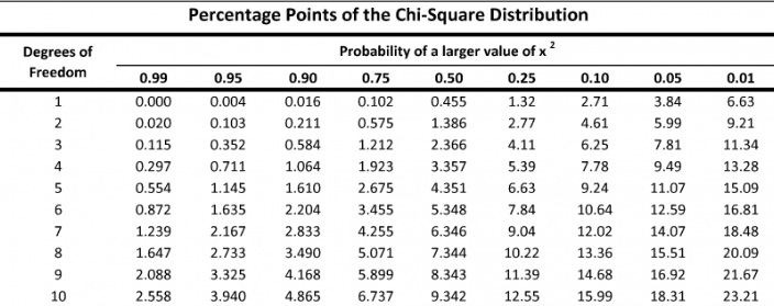
We will look at the column for one degree of freedom. Typically, scientists use a .05 critical value. A .05 critical value represents that there is a 95% chance that the difference between the data you expected to get and the data you observed is due to something other than chance. In this example, our value will be 3.84.

Coin Flip Results

In our coin flip experiment, Chi Square was 1. When we look at the table, we see that Chi Square must have been greater than 3.84 for us to say that the expected data was significantly different from the observed data. We did not reach that threshold. So, for this example, we will say that we failed to reject the null hypothesis.

The best way to get better at these statistical questions is to practice. Next, we will go through a question using the Chi Square Test that you could see on your AP® Bio exam.

AP® Biology Exam Question

This question was adapted from the 2013 AP® Biology exam.

In an investigation of fruit-fly behavior, a covered choice chamber is used to test whether the spatial distribution of flies is affected by the presence of a substance placed at one end of the chamber. To test the flies’ preference for glucose, 60 flies are introduced into the middle of the choice chamber at the insertion point. A ripe banana is placed at one end of the chamber, and an unripe banana is placed at the other end. The positions of flies are observed and recorded after 1 minute and after 10 minutes. Perform a Chi Square test on the data for the ten minute time point. Specify the null hypothesis and accept or reject it.

Okay, we will begin by identifying the null hypothesis . The null hypothesis would be that the flies would be evenly distributed across the three chambers (ripe, middle, and unripe).

Next, we will perform the Chi-Square test just like we did in the heads or tails experiment. Because there are three conditions, it may be helpful to use this set up to organize yourself:

Ok, so we have a Chi Square of 48.9. Our degrees of freedom are 3(ripe, middle, unripe)-1=2. Let’s look at that table above for a confidence variable of .05. You should get a value of 5.99. Our Chi Square value of 48.9 is much larger than 5.99 so in this case we are able to reject the null hypothesis. This means that the flies are not randomly assorting themselves, and the banana is influencing their behavior.

The Chi Square test is something that takes practice. Once you learn the system of solving these problems, you will be able to solve any Chi Square problem using the exact same method every time! In this article, we have reviewed the Chi Square test using two examples. If you are still interested in reviewing the bio-statistics that will be on your AP® Biology Exam, please check out our article The Dihybrid Cross Problem: AP® Biology Crash Course . Let us know how studying is going and if you have any questions!

Need help preparing for your AP® Biology exam?

Albert has hundreds of AP® Biology practice questions, free response, and full-length practice tests to try out.

Interested in a school license?​

Popular posts.

AP® Score Calculators

Simulate how different MCQ and FRQ scores translate into AP® scores

AP® Review Guides

The ultimate review guides for AP® subjects to help you plan and structure your prep.

Core Subject Review Guides

Review the most important topics in Physics and Algebra 1 .

SAT® Score Calculator

See how scores on each section impacts your overall SAT® score

ACT® Score Calculator

See how scores on each section impacts your overall ACT® score

Grammar Review Hub

Comprehensive review of grammar skills

AP® Posters

Download updated posters summarizing the main topics and structure for each AP® exam.

• School Guide
• Mathematics
• Number System and Arithmetic
• Trigonometry
• Probability
• Mensuration
• Maths Formulas
• Class 8 Maths Notes
• Class 9 Maths Notes
• Class 10 Maths Notes
• Class 11 Maths Notes
• Class 12 Maths Notes
• Greater Than and Less Than Symbols | Meaning of Signs and Examples
• Numerator in Mathematics
• Rational and Irrational Numbers
• Expanded Form
• Perfect Cubes - Definition, List, Chart and Examples
• Linear Algebra Symbols
• Divisibility Rule of 11
• Perfect Numbers
• Denominator in Maths
• Additive Inverse and Multiplicative Inverse
• Measurement
• Predecessor and Successor
• Binary Multiplication
• Area and Perimeter of Shapes | Formula and Examples
• Probability and Statistics
• Number Symbols
• Square Root of 4
• Factors of 30
• Binary Division

Null Hypothesis

Null Hypothesis , often denoted as H 0, is a foundational concept in statistical hypothesis testing. It represents an assumption that no significant difference, effect, or relationship exists between variables within a population. It serves as a baseline assumption, positing no observed change or effect occurring. The null is t he truth or falsity of an idea in analysis.

In this article, we will discuss the null hypothesis in detail, along with some solved examples and questions on the null hypothesis.

Table of Content

• What Is a Null Hypothesis?

Symbol of Null Hypothesis

Formula of null hypothesis, types of null hypothesis, principle of null hypothesis, how do you find null hypothesis, what is a null hypothesis.

Null Hypothesis in statistical analysis suggests the absence of statistical significance within a specific set of observed data. Hypothesis testing, using sample data, evaluates the validity of this hypothesis. Commonly denoted as H 0 or simply “null,” it plays an important role in quantitative analysis, examining theories related to markets, investment strategies, or economies to determine their validity.

Definition of Null Hypothesis

Null Hypothesis represent a default position, often suggesting no effect or difference, against which researchers compare their experimental results. The Null Hypothesis, often denoted as H 0 , asserts a default assumption in statistical analysis. It posits no significant difference or effect, serving as a baseline for comparison in hypothesis testing.

Null Hypothesis is represented as H 0 , the Null Hypothesis symbolizes the absence of a measurable effect or difference in the variables under examination.

Certainly, a simple example would be asserting that the mean score of a group is equal to a specified value like stating that the average IQ of a population is 100.

The Null Hypothesis is typically formulated as a statement of equality or absence of a specific parameter in the population being studied. It provides a clear and testable prediction for comparison with the alternative hypothesis. The formulation of the Null Hypothesis typically follows a concise structure, stating the equality or absence of a specific parameter in the population.

Mean Comparison (Two-sample t-test)

H 0 : μ 1 = μ 2

This asserts that there is no significant difference between the means of two populations or groups.

Proportion Comparison

H 0 : p 1 − p 2 = 0

This suggests no significant difference in proportions between two populations or conditions.

Equality in Variance (F-test in ANOVA)

H 0 : σ 1 = σ 2

This states that there’s no significant difference in variances between groups or populations.

Independence (Chi-square Test of Independence):

H 0 : Variables are independent

This asserts that there’s no association or relationship between categorical variables.

Null Hypotheses vary including simple and composite forms, each tailored to the complexity of the research question. Understanding these types is pivotal for effective hypothesis testing.

Equality Null Hypothesis (Simple Null Hypothesis)

The Equality Null Hypothesis, also known as the Simple Null Hypothesis, is a fundamental concept in statistical hypothesis testing that assumes no difference, effect or relationship between groups, conditions or populations being compared.

Non-Inferiority Null Hypothesis

In some studies, the focus might be on demonstrating that a new treatment or method is not significantly worse than the standard or existing one.

Superiority Null Hypothesis

The concept of a superiority null hypothesis comes into play when a study aims to demonstrate that a new treatment, method, or intervention is significantly better than an existing or standard one.

Independence Null Hypothesis

In certain statistical tests, such as chi-square tests for independence, the null hypothesis assumes no association or independence between categorical variables.

Homogeneity Null Hypothesis

In tests like ANOVA (Analysis of Variance), the null hypothesis suggests that there’s no difference in population means across different groups.

Examples of Null Hypothesis

• Medicine: Null Hypothesis: “No significant difference exists in blood pressure levels between patients given the experimental drug versus those given a placebo.”
• Education: Null Hypothesis: “There’s no significant variation in test scores between students using a new teaching method and those using traditional teaching.”
• Economics: Null Hypothesis: “There’s no significant change in consumer spending pre- and post-implementation of a new taxation policy.”
• Environmental Science: Null Hypothesis: “There’s no substantial difference in pollution levels before and after a water treatment plant’s establishment.”

The principle of the null hypothesis is a fundamental concept in statistical hypothesis testing. It involves making an assumption about the population parameter or the absence of an effect or relationship between variables.

In essence, the null hypothesis (H 0 ) proposes that there is no significant difference, effect, or relationship between variables. It serves as a starting point or a default assumption that there is no real change, no effect or no difference between groups or conditions.

Null Hypothesis Rejection

Rejecting the Null Hypothesis occurs when statistical evidence suggests a significant departure from the assumed baseline. It implies that there is enough evidence to support the alternative hypothesis, indicating a meaningful effect or difference. Null Hypothesis rejection occurs when statistical evidence suggests a deviation from the assumed baseline, prompting a reconsideration of the initial hypothesis.

Identifying the Null Hypothesis involves defining the status quotient, asserting no effect and formulating a statement suitable for statistical analysis.

When is Null Hypothesis Rejected?

The Null Hypothesis is rejected when statistical tests indicate a significant departure from the expected outcome, leading to the consideration of alternative hypotheses. It occurs when statistical evidence suggests a deviation from the assumed baseline, prompting a reconsideration of the initial hypothesis.

Null Hypothesis and Alternative Hypothesis

In the realm of hypothesis testing, the null hypothesis (H 0 ) and alternative hypothesis (H₁ or Ha) play critical roles. The null hypothesis generally assumes no difference, effect, or relationship between variables, suggesting that any observed change or effect is due to random chance. Its counterpart, the alternative hypothesis, asserts the presence of a significant difference, effect, or relationship between variables, challenging the null hypothesis. These hypotheses are formulated based on the research question and guide statistical analyses.

Null Hypothesis vs Alternative Hypothesis

The null hypothesis (H 0 ) serves as the baseline assumption in statistical testing, suggesting no significant effect, relationship, or difference within the data. It often proposes that any observed change or correlation is merely due to chance or random variation. Conversely, the alternative hypothesis (H 1 or Ha) contradicts the null hypothesis, positing the existence of a genuine effect, relationship or difference in the data. It represents the researcher’s intended focus, seeking to provide evidence against the null hypothesis and support for a specific outcome or theory. These hypotheses form the crux of hypothesis testing, guiding the assessment of data to draw conclusions about the population being studied.

Example of Alternative and Null Hypothesis

Let’s envision a scenario where a researcher aims to examine the impact of a new medication on reducing blood pressure among patients. In this context:

Null Hypothesis (H 0 ): “The new medication does not produce a significant effect in reducing blood pressure levels among patients.”

Alternative Hypothesis (H 1 or Ha): “The new medication yields a significant effect in reducing blood pressure levels among patients.”

The null hypothesis implies that any observed alterations in blood pressure subsequent to the medication’s administration are a result of random fluctuations rather than a consequence of the medication itself. Conversely, the alternative hypothesis contends that the medication does indeed generate a meaningful alteration in blood pressure levels, distinct from what might naturally occur or by random chance.

Also, Check

Solved Examples on Null Hypothesis

Example 1: A researcher claims that the average time students spend on homework is 2 hours per night.

Null Hypothesis (H 0 ): The average time students spend on homework is equal to 2 hours per night. Data: A random sample of 30 students has an average homework time of 1.8 hours with a standard deviation of 0.5 hours. Test Statistic and Decision: Using a t-test, if the calculated t-statistic falls within the acceptance region, we fail to reject the null hypothesis. If it falls in the rejection region, we reject the null hypothesis. Conclusion: Based on the statistical analysis, we fail to reject the null hypothesis, suggesting that there is not enough evidence to dispute the claim of the average homework time being 2 hours per night.

Example 2: A company asserts that the error rate in its production process is less than 1%.

Null Hypothesis (H 0 ): The error rate in the production process is 1% or higher. Data: A sample of 500 products shows an error rate of 0.8%. Test Statistic and Decision: Using a z-test, if the calculated z-statistic falls within the acceptance region, we fail to reject the null hypothesis. If it falls in the rejection region, we reject the null hypothesis. Conclusion: The statistical analysis supports rejecting the null hypothesis, indicating that there is enough evidence to dispute the company’s claim of an error rate of 1% or higher.

Null Hypothesis – Practice Problems

Q1. A researcher claims that the average time spent by students on homework is less than 2 hours per day. Formulate the null hypothesis for this claim?

Q2. A manufacturing company states that their new machine produces widgets with a defect rate of less than 5%. Write the null hypothesis to test this claim?

Q3. An educational institute believes that their online course completion rate is at least 60%. Develop the null hypothesis to validate this assertion?

Q4. A restaurant claims that the waiting time for customers during peak hours is not more than 15 minutes. Formulate the null hypothesis for this claim?

Q5. A study suggests that the mean weight loss after following a specific diet plan for a month is more than 8 pounds. Construct the null hypothesis to evaluate this statement?

Null Hypothesis – Frequently Asked Questions

How to form a null hypothesis.

A null hypothesis is formed based on the assumption that there is no significant difference or effect between the groups being compared or no association between variables being tested. It often involves stating that there is no relationship, no change, or no effect in the population being studied.

When Do we reject the Null Hypothesis?

In statistical hypothesis testing, if the p-value (the probability of obtaining the observed results) is lower than the chosen significance level (commonly 0.05), we reject the null hypothesis. This suggests that the data provides enough evidence to refute the assumption made in the null hypothesis.

What is a Null Hypothesis in Research?

In research, the null hypothesis represents the default assumption or position that there is no significant difference or effect. Researchers often try to test this hypothesis by collecting data and performing statistical analyses to see if the observed results contradict the assumption.

What Are Alternative and Null Hypotheses?

The null hypothesis (H0) is the default assumption that there is no significant difference or effect. The alternative hypothesis (H1 or Ha) is the opposite, suggesting there is a significant difference, effect or relationship.

What Does it Mean to Reject the Null Hypothesis?

Rejecting the null hypothesis implies that there is enough evidence in the data to support the alternative hypothesis. In simpler terms, it suggests that there might be a significant difference, effect or relationship between the groups or variables being studied.

How to Find Null Hypothesis?

Formulating a null hypothesis often involves considering the research question and assuming that no difference or effect exists. It should be a statement that can be tested through data collection and statistical analysis, typically stating no relationship or no change between variables or groups.

How is Null Hypothesis denoted?

The null hypothesis is commonly symbolized as H 0 in statistical notation.

What is the Purpose of the Null hypothesis in Statistical Analysis?

The null hypothesis serves as a starting point for hypothesis testing, enabling researchers to assess if there’s enough evidence to reject it in favor of an alternative hypothesis.

What happens if we Reject the Null hypothesis?

Rejecting the null hypothesis implies that there is sufficient evidence to support an alternative hypothesis, suggesting a significant effect or relationship between variables.

Is it Possible to Prove the Null Hypothesis?

No, statistical testing aims to either reject or fail to reject the null hypothesis based on evidence from sample data. It does not prove the null hypothesis to be true.

What are Test for Null Hypothesis?

Various statistical tests, such as t-tests or chi-square tests, are employed to evaluate the validity of the Null Hypothesis in different scenarios.

Please Login to comment...

Similar reads.

• Geeks Premier League 2023
• Math-Concepts
• Geeks Premier League
• School Learning
• 10 Ways to Use Microsoft OneNote for Note-Taking
• 10 Best Yellow.ai Alternatives & Competitors in 2024
• 10 Best Online Collaboration Tools 2024
• 10 Best Autodesk Maya Alternatives for 3D Animation and Modeling in 2024
• 30 OOPs Interview Questions and Answers (2024)

Improve your Coding Skills with Practice

What kind of Experience do you want to share?