research article on global warming

Climate Change

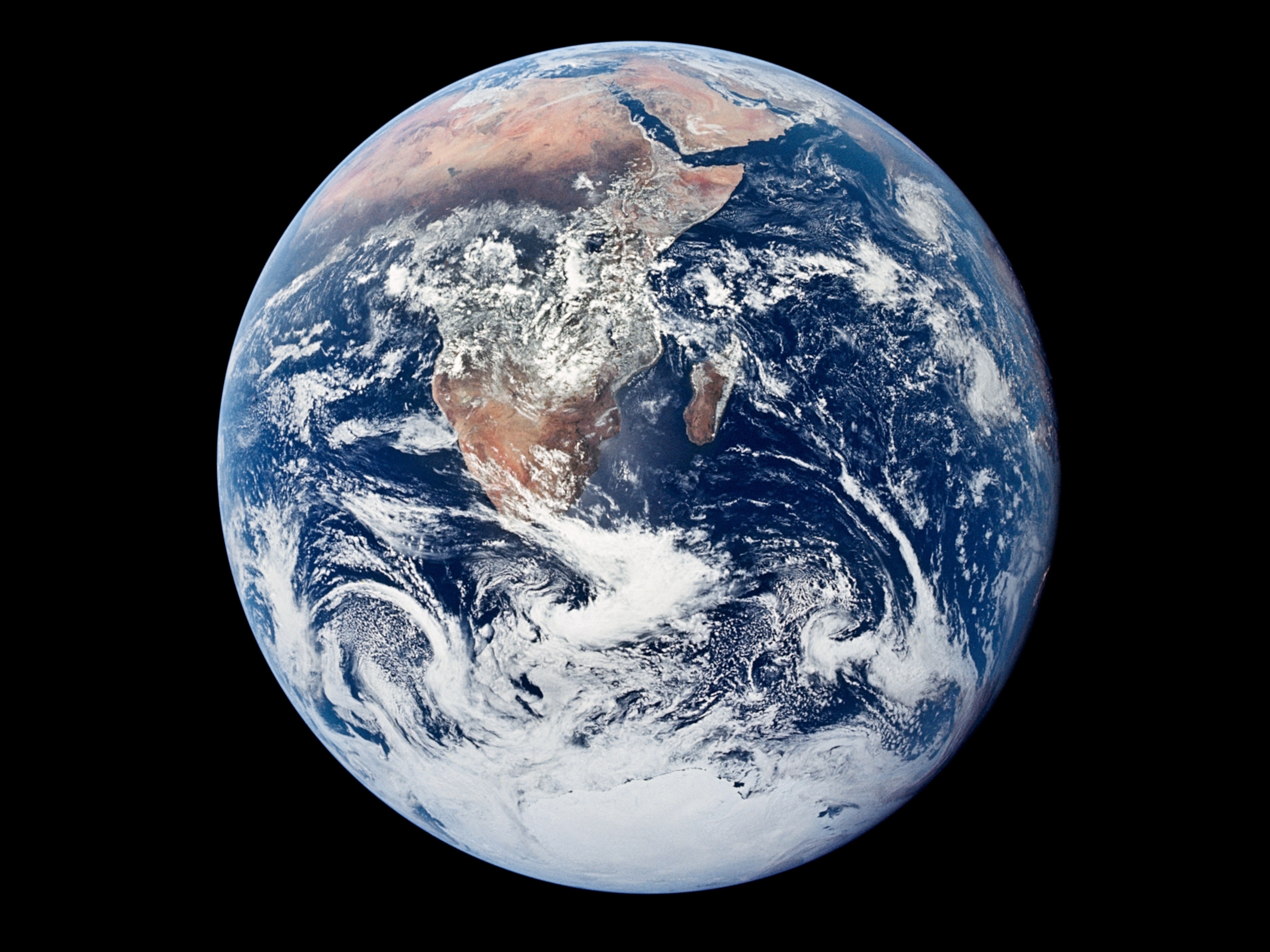
From the unique vantage point in space, NASA collects critical long-term observations of our changing planet.

Latest News

NASA Data Helps Beavers Build Back Streams

NASA Selects New Aircraft-Driven Studies of Earth and Climate Change

Climate Change Research

NASA Open Science Initiative Expands OpenET Across Amazon Basin  

How NASA Spotted El Niño Changing the Saltiness of Coastal Waters

How Do We Know Climate Change is Real?

There is unequivocal evidence that Earth is warming at an unprecedented rate. Human activity is the principal cause.

Earth-orbiting satellites and new technologies have helped scientists see the big picture, collecting many different types of information about our planet and its climate all over the world. These data, collected over many years, reveal the signs and patterns of a changing climate.

What is causing climate change?

Human activities are driving the global warming trend observed since the mid-20th century.

Scientists attribute the global warming trend observed since the mid-20 th century to the human expansion of the "greenhouse effect" — warming that results when the atmosphere traps heat radiating from Earth toward space. Over the last century, burning of fossil fuels like coal and oil has increased the concentration of atmospheric carbon dioxide (CO 2 ). This increase happens because the coal or oil burning process combines carbon with oxygen in the air to make CO 2 .

What are the effects of climate change?

The effects of human-caused global warming are happening now, are irreversible for people alive today, and will worsen as long as humans add greenhouse gases to the atmosphere.

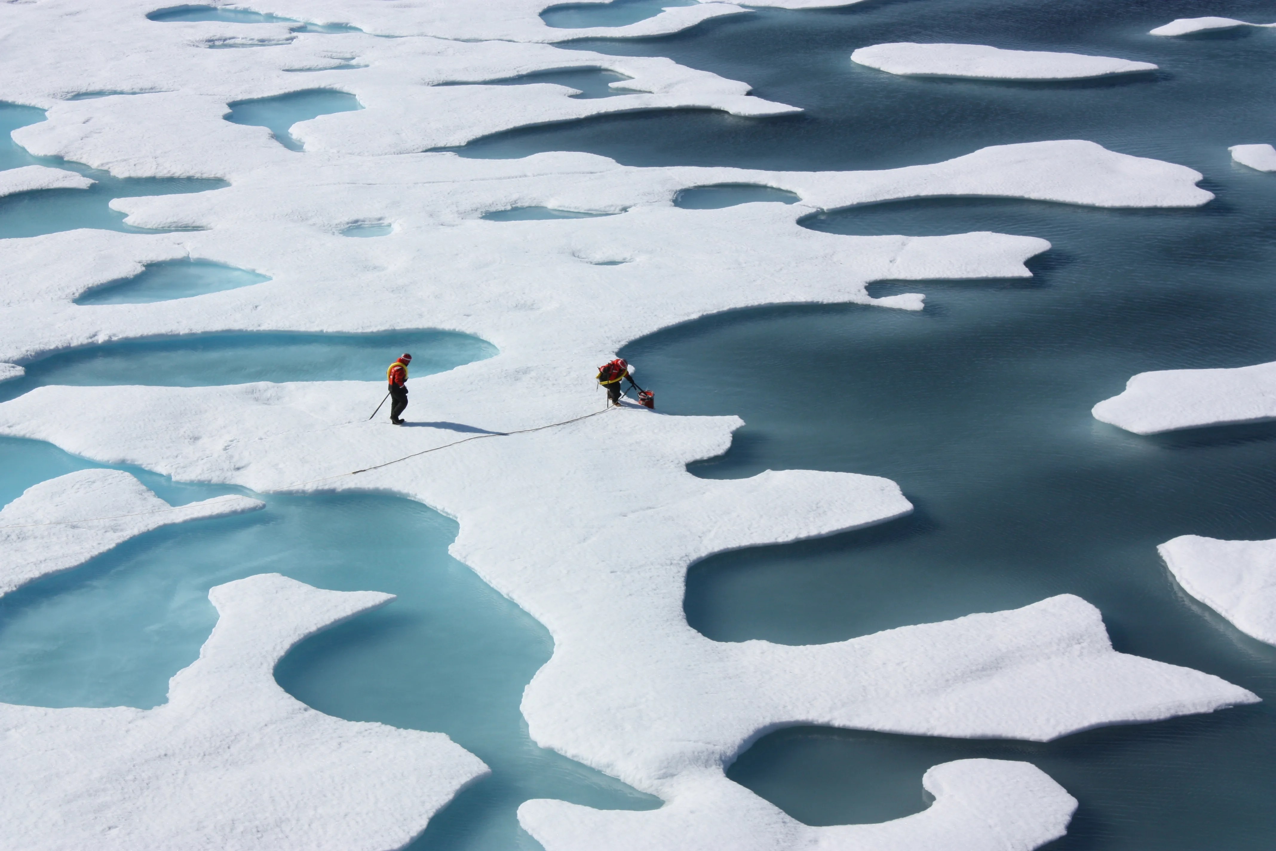
We already see effects scientists predicted, such as the loss of sea ice, melting glaciers and ice sheets, sea level rise, and more intense heat waves. Scientists predict global temperature increases from human-made greenhouse gases will continue. Severe weather damage will also increase and intensify.

Images of Change

Before-and-after images of Earth.

Climate Change Resources

Climate Time Machine

Climate change in recent history

Global Ice Viewer

Climate change’s impact on ice

Vast library of images, videos, graphics, and more

Creciente biblioteca de recursos en español

Climate Data Resources

Sea Level Change Observations from Space

Established in 2014, this NASA-sponsored team works to improve the understanding of regional relative sea-level change on a range of timescales. They work with partners to translate the latest science and research into actionable information  and to communicate how impacts are increasing at the coast.

NASA Center for Climate Simulation (NCCS)

NCCS provides high performance computing for NASA-sponsored scientists and engineers. The purpose  is to enhance NASA capabilities in Earth science, with an emphasis on weather and climate prediction, and to enable future scientific discoveries that will benefit humankind.

GISS Surface Temperature Analysis (GISTEMP)

NASA’s Goddard Institute of Space Studies assembles one of the world's most trusted global temperature records, using a combination of surface air temperature data acquired by tens of thousands of meteorological stations, as well as sea surface temperature data from ship- and buoy-based instruments.

NASA Earth Exchange (NEX)

NEX combines state-of-the-art supercomputing, Earth system modeling, and NASA remote sensing data feeds to deliver a work environment for exploring and analyzing terabyte- to petabyte-scale datasets covering large regions, continents or the globe.

Global Modeling and Assimilation Office (GMAO)

GMAO members perform research, develop models and assimilation systems, and produce quasi-operational products in support of NASA's missions. The Goddard Earth Observing System" (GEOS) family of models is used for applications across a wide range of spatial scales, from kilometers to many tens of kilometers. 

World of Change

NASA Earth Observatory has produced a collection of image series that show some features of Earth that have changed over time due to both natural and human-induced causes.

Knowledge is power

Stay in the know about climate impacts and solutions. Subscribe to our weekly newsletter.

By clicking submit, you agree to share your email address with the site owner and Mailchimp to receive emails from the site owner. Use the unsubscribe link in those emails to opt out at any time.

Yale Climate Connections

Scientists agree: Climate change is real and caused by people

Share this:

• Click to share on Facebook (Opens in new window)
• Click to share on X (Opens in new window)

[Leer en español aquí]

The scientific consensus that climate change is happening and that it is human-caused is strong. Scientific investigation of global warming began in the 19th century , and by the early 2000s, this research began to coalesce into confidence about the reality, causes, and general range of adverse effects of global warming. This conclusion was drawn from studying air and ocean temperatures, the atmosphere’s composition, satellite records, ice cores, modeling, and more.

In 1988 the United Nations and World Meteorological Organization founded the Intergovernmental Panel on Climate Change, IPCC, to provide regular updates on the scientific evidence on global warming. In a 2013 report , the IPCC concluded that scientific evidence of warming is “unequivocal” and that the largest cause is an increase of carbon dioxide in the atmosphere as a result of humans burning fossil fuels. The IPCC continues to assess this science, periodically issuing new reports.

Climate change is real and caused by humans

The IPCC is not the only scientific group that has reached a clear consensus on the scientific evidence of human-caused global warming. As this NASA page points out, 200 global scientific organizations, 11 international science academies, and 18 American science associations have released statements in alignment with this consensus.

Amanda Staudt is the senior director for climate, atmospheric and polar sciences at the National Academies of Science, Engineering and Medicine, where she has worked since 2001. The Academies, she said, first began studying climate change in 1979, researching how much warming would likely happen if the amount of carbon dioxide concentrations in the atmosphere were doubled.

Four decades later, those findings have held up and have been strengthened based on scores of continued studies and analysis. “The remarkable thing about that study,” she said, “is that they basically got the right answer” from the start. This 1979 study by the National Research Council, Staudt said, led to investment in climate science in the U.S. 

Though this consensus has been thoroughly established, scientific research and new findings continue. Staudt said countless attempted rebuttals of climate science findings have been researched and disproved.

“We did a lot of studies in that time period, looking at those questions,” she said, ”and one by one, putting them to bed and convincing ourselves over and over again, that humans were affecting climate, and that we could document that effect.”

At the National Academies, reaching consensus requires open sessions and dialogue with scientists and agreement from committees, which typically consist of 12-15 experts. Their draft reports go through peer review, and reviewers’ concerns are resolved before publication is approved. The goal is for the complex science of climate change to become as thoroughly researched and substantiated as possible.

“One of the things I think about scientists is that we’re all inherently skeptics at some level,” Staudt said. “That’s what drives us to science, that we have questions about the world around us. And we want to prove that for ourselves.”

Scientists consistently reaffirm evidence that climate change is happening

Climate scientists worldwide go through similar processes before their findings are published. And their research papers, too, show a strong consensus about global warming. As NASA states on its website , “Multiple studies published in peer-reviewed scientific journals show that 97 percent or more of actively publishing climate scientists agree: Climate-warming trends over the past century are extremely likely due to human activities.” (By sound practice, scientists resist saying science is for all times “certain” or that its findings are “final,” and the “extremely likely” language respects that practice.)

One of the studies about the consensus was led by John Cook, a fellow at the Climate Change Communication Research Hub at Monash University in Melbourne, Australia. Cook and colleagues reviewed nearly 12,000 scientific papers to examine how aligned published research is on major findings on climate change. That study found that 97 percent of scholarly papers that take a position on climate change do endorse the consensus. The papers that rejected the consensus position contained errors, according to subsequent research .

In reviewing the papers, Cook has said he and his colleagues found the consensus to have been so widely accepted by 2013 that many researchers by then no longer felt a need to mention or reaffirm it in their research papers.

Also see: Causes of global warming: How scientists know that humans are responsible

Samantha Harrington

Samantha Harrington, director of audience experience for Yale Climate Connections, is a journalist and graphic designer with a background in digital media and entrepreneurship. Sam is especially interested... More by Samantha Harrington

Suggested Searches

Climate change.

• Expedition 64
• Mars perseverance
• SpaceX Crew-2
• International Space Station
• View All Topics A-Z

Humans in Space

Earth & climate, the solar system, the universe, aeronautics, learning resources, news & events.

Join NASA in Celebrating Earth Day 2024 by Sharing a #GlobalSelfie

NASA Selects New Aircraft-Driven Studies of Earth and Climate Change

The Ocean Touches Everything: Celebrate Earth Day with NASA

• Search All NASA Missions
• A to Z List of Missions
• Upcoming Launches and Landings
• Spaceships and Rockets
• Communicating with Missions
• James Webb Space Telescope
• Hubble Space Telescope
• Why Go to Space
• Astronauts Home
• Commercial Space
• Destinations
• Living in Space
• Explore Earth Science
• Earth, Our Planet
• Earth Science in Action
• Earth Multimedia
• Earth Science Researchers
• Pluto & Dwarf Planets
• Asteroids, Comets & Meteors
• The Kuiper Belt
• The Oort Cloud
• Skywatching
• The Search for Life in the Universe
• Black Holes
• The Big Bang
• Dark Energy & Dark Matter
• Earth Science
• Planetary Science
• Astrophysics & Space Science
• The Sun & Heliophysics
• Biological & Physical Sciences
• Lunar Science
• Citizen Science
• Astromaterials
• Aeronautics Research
• Human Space Travel Research
• Science in the Air
• NASA Aircraft
• Flight Innovation
• Supersonic Flight
• Air Traffic Solutions
• Green Aviation Tech
• Drones & You
• Technology Transfer & Spinoffs
• Space Travel Technology
• Technology Living in Space
• Manufacturing and Materials
• Science Instruments
• For Kids and Students
• For Educators
• For Colleges and Universities
• For Professionals
• Science for Everyone
• Requests for Exhibits, Artifacts, or Speakers
• STEM Engagement at NASA
• NASA's Impacts
• Centers and Facilities
• Directorates
• Organizations
• People of NASA
• Internships
• Our History
• Doing Business with NASA
• Get Involved
• Aeronáutica
• Ciencias Terrestres
• Sistema Solar
• All NASA News
• Video Series on NASA+
• Newsletters
• Social Media
• Media Resources
• Upcoming Launches & Landings
• Virtual Events
• Sounds and Ringtones
• Interactives
• STEM Multimedia

Work Underway on Large Cargo Landers for NASA’s Artemis Moon Missions

Mars Science Laboratory: Curiosity Rover

NASA Open Science Initiative Expands OpenET Across Amazon Basin  

NASA Motion Sickness Study Volunteers Needed!

Students Celebrate Rockets, Environment at NASA’s Kennedy Space Center

AI for Earth: How NASA’s Artificial Intelligence and Open Science Efforts Combat Climate Change

Sols 4159-4160: A Fully Loaded First Sol

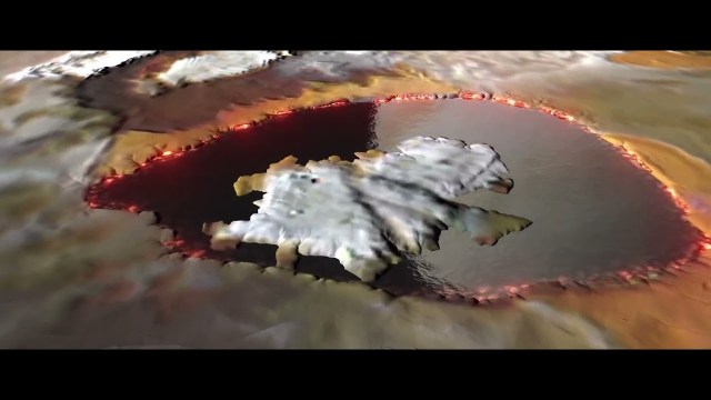
NASA’s Juno Gives Aerial Views of Mountain, Lava Lake on Io

Hubble Captures a Bright Galactic and Stellar Duo

NASA’s TESS Returns to Science Operations

Astronauts To Patch Up NASA’s NICER Telescope

Hubble Goes Hunting for Small Main Belt Asteroids

NASA’s Near Space Network Enables PACE Climate Mission to ‘Phone Home’

NASA Photographer Honored for Thrilling Inverted In-Flight Image

NASA Langley Team to Study Weather During Eclipse Using Uncrewed Vehicles

ARMD Solicitations

Amendment 10: B.9 Heliophysics Low-Cost Access to Space Final Text and Proposal Due Date.

Tech Today: Taking Earth’s Pulse with NASA Satellites

Earth Day 2024: Posters and Virtual Backgrounds

NASA Names Finalists of the Power to Explore Challenge

Diez maneras en que los estudiantes pueden prepararse para ser astronautas

Astronauta de la NASA Marcos Berríos

Resultados científicos revolucionarios en la estación espacial de 2023

Climate change research.

Science in Space: April 2024

Everyone on Earth is touched by the effects of climate change, such as hotter temperatures, shifts in rain patterns, and sea level rise. Collecting climate data helps communities better plan for these changes and build more resilience to them.

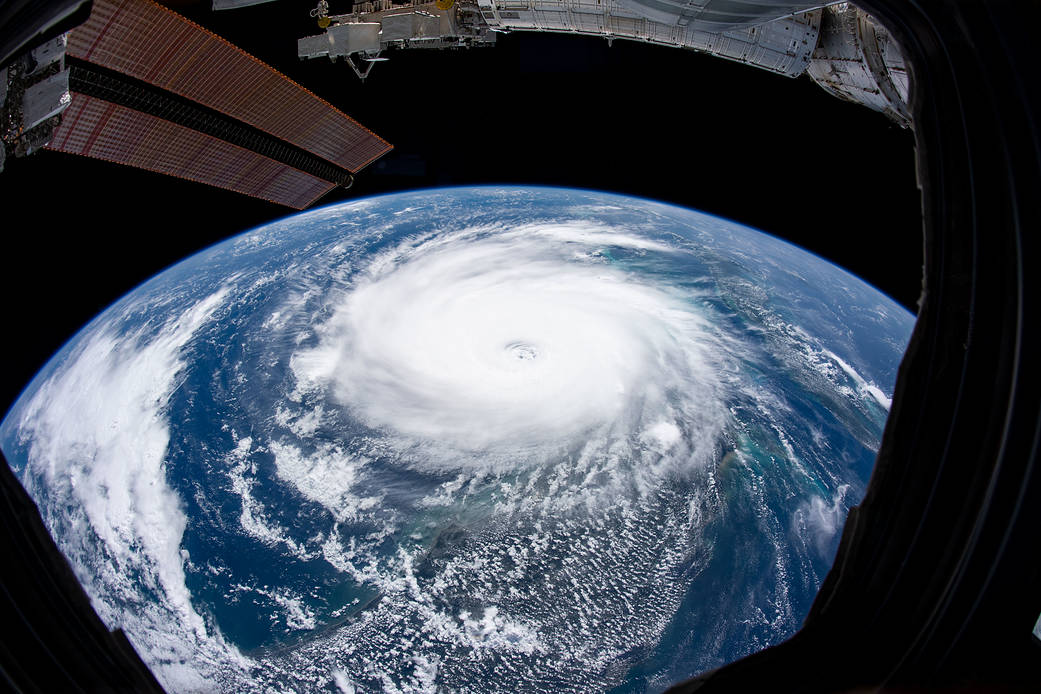
The International Space Station, one of dozens of NASA missions contributing to this effort, has multiple instruments collecting various types of climate-related data. Because the station’s orbit passes over 90 percent of Earth’s population and circles the planet 16 times each day, these instruments have views of multiple locations at different times of day and night. The data inform climate decisions and help scientists understand and solve the challenges created by climate change.

While crew members have little involvement in the ongoing operation of these instruments, they do play a critical role in unpacking hardware when it arrives at the space station and in assembling and installing the instruments via spacewalks or using the station’s robotic arm.

One investigation on the orbiting lab that contributes to efforts to monitor and address climate change is ECOsystem Spaceborne Thermal Radiometer Experiment on Space Station ( ECOSTRESS ). It provides thermal infrared measurements of Earth’s surface that help answer questions about water stress in plants and how specific regions respond to climate change. Research confirmed the accuracy of ECOSTRESS surface estimates 1 and found that the process of photosynthesis in plants begins to fail at 46.7 degrees C (114 degrees F). 2 Average temperatures have increased 0.5 degrees C per decade in some tropical regions, and temperature extremes are becoming more pronounced. Rainforests are a primary producer of oxygen and, without sufficient mitigation of the effects of climate change, leaf temperatures in these tropical forests soon could approach this failure threshold.

The Total and Spectral Solar Irradiance Sensor ( TSIS ) measures total solar irradiance (TSI) and solar spectral irradiance (SSI). TSI is the total solar energy input to Earth and SSI measures the Sun’s energy in individual wavelengths. Energy from the Sun drives atmospheric and oceanic circulations on Earth, and knowing its magnitude and variability is essential to understanding Earth’s climate. Researchers verified the instrument’s performance and showed that it made more accurate measurements than previous instruments. 3,4 TSIS maintains a continuity of nearly 40 years of data on solar irradiance from space-based observations.

To view this video please enable JavaScript, and consider upgrading to a web browser that supports HTML5 video

The Global Ecosystem Dynamics Investigation ( GEDI ) observes global forests and topography using light detection and ranging (lidar). These observations could provide insight into important carbon and water cycling processes, biodiversity, and habitat. One study used GEDI data to estimate pan-tropical and temperate biomass densities at the national level for every country observed and the sub-national level for the United States. 5

Earth Surface Mineral Dust Source Investigation ( EMIT ) determines the type and distribution of minerals in the dust of Earth’s arid regions using an imaging spectrometer. Mineral dust affects local warming and cooling, air quality, rate of snow melt, and ocean plankton growth. Researchers demonstrated that data from EMIT also can be used to identify and monitor specific sources of methane and carbon dioxide emissions. Carbon dioxide and methane are the primary human-caused drivers of climate change. Increasing emissions in areas with poor reporting requirements create significant uncertainty in the global carbon budget. 6 The high spatial resolution of EMIT data could allow precise monitoring even of sources that are close together.

The station’s Orbiting Carbon Observatory-3 ( OCO-3 ) collects data on global carbon dioxide during sunlit hours, mapping emissions of targeted local hotspots. This type of satellite-based remote sensing helps assess and verify emission reductions included in national and global plans and agreements. Monitoring by OCO-3 and the Italian Space Agency’s PRecursore IperSpettrale della Missione Applicativa (PRISMA) satellite of 30 coal-fired power plants between 2021 and 2022 showed agreement with on-site observations. 7 This result suggests that under the right conditions, satellites can provide reliable estimates of emissions from discreet sources. Combustion for power and other industrial uses account for an estimated 59% of global human-caused carbon dioxide emissions.

The Stratospheric Aerosol and Gas Experiment III-ISS ( SAGE III-ISS ) measures ozone and other gases and tiny particles in the atmosphere, called aerosols, that together act as Earth’s sunscreen. The instrument can distinguish between clouds and aerosols in the atmosphere. A study showed that aerosols dominate Earth’s tropical upper troposphere and lower stratosphere, a transition region between the two atmospheric levels. Continuous monitoring and identification of these layers of the atmosphere helps quantify their effect on Earth’s climate. 8

An early remote sensing system, ISS SERVIR Environmental Research and Visualization System ( ISERV ), automatically took images of Earth to help scientists assess and monitor disasters and other significant events. Researchers reported that this type of Earth observation is critical for applications such as mapping land use and assessing carbon biomass and ocean health. 9

John Love, ISS Research Planning Integration Scientist Expedition 71

Search this database of scientific experiments to learn more about those mentioned above.

1 Weidberg N, Lopez Chiquillo L, Roman S, Roman M, Vazquez E, et al. Assessing high resolution thermal monitoring of complex intertidal environments from space: The case of ECOSTRESS at Rias Baixas, NW Iberia. Remote Sensing Applications: Society and Environment. 2023 November; 32101055. DOI: 10.1016/j.rsase.2023.101055.

2 Doughty CE, Keany JM, Wiebe BC, Rey-Sanchez C, Carter KR, et al. Tropical forests are approaching critical temperature thresholds. Nature. 2023 August 23; 621105-111. DOI: 10.1038/s41586-023-06391-z.

3 Richard EC, Harber D, Coddington OM, Drake G, Rutkowski J, et al. SI-traceable spectral irradiance radiometric characterization and absolute calibration of the TSIS-1 Spectral Irradiance Monitor (SIM). Remote Sensing. 2020 January; 12(11): 1818. DOI:  10.3390/rs12111818.

4 Coddington OM, Richard EC, Harber D, Pilewskie P, Chance K, et al. The TSIS-1 hybrid solar reference spectrum. Geophysical Research Letters. 2021 April 26; 48(12): e2020GL091709. DOI:  10.1029/2020GL091709

5 Dubayah R, Armston J, Healey S, Bruening JM, Patterson PL, et al. GEDI launches a new era of biomass inference from space. Environmental Research Letters. 2022 August; 17(9): 095001. DOI: 10.1088/1748-9326/ac8694.

6 Thorpe A, Green RD, Thompson DR, Brodrick PG, Chapman DK, et al. Attribution of individual methane and carbon dioxide emission sources using EMIT observations from space. Science Advances. 2023 November 17; 9(46): eadh2391. DOI: 10.1126/sciadv.adh2391.

7 Cusworth DH, Thorpe A, Miller CE, Ayasse AK, Jiorle R, et al. Two years of satellite-based carbon dioxide emission quantification at the world’s largest coal-fired power plants. Atmospheric Chemistry and Physics. 2023 November 24; 23(22): 14577-14591. DOI: 10.5194/acp-23-14577-2023.

8 Bhatta S, Pandit AK, Loughman R, Vernier J. Three-wavelength approach for aerosol-cloud discrimination in the SAGE III/ISS aerosol extinction dataset. Applied Optics. 2023 May; 62(13): 3454-3466. DOI: 10.1364/AO.485466 .

9 Kansakar P, Hossain F. A review of applications of satellite earth observation data for global societal benefit and stewardship of planet earth. Space Policy. 2016 May; 3646-54.

Discover More Topics

Latest News from Space Station Research

Station Science 101: Earth and Space Science

NASA is a global leader in studying Earth’s changing climate.

Space Station Research and Technology

ENCYCLOPEDIC ENTRY

Global warming.

The causes, effects, and complexities of global warming are important to understand so that we can fight for the health of our planet.

Earth Science, Climatology

Tennessee Power Plant

Ash spews from a coal-fueled power plant in New Johnsonville, Tennessee, United States.

Photograph by Emory Kristof/ National Geographic

Global warming is the long-term warming of the planet’s overall temperature. Though this warming trend has been going on for a long time, its pace has significantly increased in the last hundred years due to the burning of fossil fuels . As the human population has increased, so has the volume of fossil fuels burned. Fossil fuels include coal, oil, and natural gas, and burning them causes what is known as the “greenhouse effect” in Earth’s atmosphere.

The greenhouse effect is when the sun’s rays penetrate the atmosphere, but when that heat is reflected off the surface cannot escape back into space. Gases produced by the burning of fossil fuels prevent the heat from leaving the atmosphere. These greenhouse gasses are carbon dioxide , chlorofluorocarbons, water vapor , methane , and nitrous oxide . The excess heat in the atmosphere has caused the average global temperature to rise overtime, otherwise known as global warming.

Global warming has presented another issue called climate change. Sometimes these phrases are used interchangeably, however, they are different. Climate change refers to changes in weather patterns and growing seasons around the world. It also refers to sea level rise caused by the expansion of warmer seas and melting ice sheets and glaciers . Global warming causes climate change, which poses a serious threat to life on Earth in the forms of widespread flooding and extreme weather. Scientists continue to study global warming and its impact on Earth.

Media Credits

The audio, illustrations, photos, and videos are credited beneath the media asset, except for promotional images, which generally link to another page that contains the media credit. The Rights Holder for media is the person or group credited.

Production Managers

Program specialists, last updated.

February 21, 2024

User Permissions

For information on user permissions, please read our Terms of Service. If you have questions about how to cite anything on our website in your project or classroom presentation, please contact your teacher. They will best know the preferred format. When you reach out to them, you will need the page title, URL, and the date you accessed the resource.

If a media asset is downloadable, a download button appears in the corner of the media viewer. If no button appears, you cannot download or save the media.

Text on this page is printable and can be used according to our Terms of Service .

Interactives

Any interactives on this page can only be played while you are visiting our website. You cannot download interactives.

Related Resources

• ENVIRONMENT

How global warming is disrupting life on Earth

The signs of global warming are everywhere, and are more complex than just climbing temperatures.

Our planet is getting hotter. Since the Industrial Revolution—an event that spurred the use of fossil fuels in everything from power plants to transportation—Earth has warmed by 1 degree Celsius, about 2 degrees Fahrenheit.  

That may sound insignificant, but 2023 was the hottest year on record , and all 10 of the hottest years on record have occurred in the past decade.  

Global warming and climate change are often used interchangeably as synonyms, but scientists prefer to use “climate change” when describing the complex shifts now affecting our planet’s weather and climate systems.  

Climate change encompasses not only rising average temperatures but also natural disasters, shifting wildlife habitats, rising seas , and a range of other impacts. All of these changes are emerging as humans continue to add heat-trapping greenhouse gases , like carbon dioxide and methane, to the atmosphere.

What causes global warming?

When fossil fuel emissions are pumped into the atmosphere, they change the chemistry of our atmosphere, allowing sunlight to reach the Earth but preventing heat from being released into space. This keeps Earth warm, like a greenhouse, and this warming is known as the greenhouse effect .  

Carbon dioxide is the most commonly found greenhouse gas and about 75 percent of all the climate warming pollution in the atmosphere. This gas is a product of producing and burning oil, gas, and coal. About a quarter of Carbon dioxide also results from land cleared for timber or agriculture.  

Methane is another common greenhouse gas. Although it makes up only about 16 percent of emissions, it's roughly 25 times more potent than carbon dioxide and dissipates more quickly. That means methane can cause a large spark in warming, but ending methane pollution can also quickly limit the amount of atmospheric warming. Sources of this gas include agriculture (mostly livestock), leaks from oil and gas production, and waste from landfills.  

What are the effects of global warming?  

One of the most concerning impacts of global warming is the effect warmer temperatures will have on Earth's polar regions and mountain glaciers. The Arctic is warming four times faster than the rest of the planet. This warming reduces critical ice habitat and it disrupts the flow of the jet stream, creating more unpredictable weather patterns around the globe.  

( Learn more about the jet stream. )

A warmer planet doesn't just raise temperatures. Precipitation is becoming more extreme as the planet heats. For every degree your thermometer rises, the air holds about seven percent more moisture. This increase in moisture in the atmosphere can produce flash floods, more destructive hurricanes, and even paradoxically, stronger snow storms.  

The world's leading scientists regularly gather to review the latest research on how the planet is changing. The results of this review is synthesized in regularly published reports known as the Intergovernmental Panel on Climate Change (IPCC) reports.  

A recent report outlines how disruptive a global rise in temperature can be:

• Coral reefs are now a highly endangered ecosystem. When corals face environmental stress, such as high heat, they expel their colorful algae and turn a ghostly white, an effect known as coral bleaching . In this weakened state, they more easily die.  
• Trees are increasingly dying from drought , and this mass mortality is reshaping forest ecosystems.
• Rising temperatures and changing precipitation patterns are making wildfires more common and more widespread. Research shows they're even moving into the eastern U.S. where fires have historically been less common.
• Hurricanes are growing more destructive and dumping more rain, an effect that will result in more damage. Some scientists say we even need to be preparing for Cat 6 storms . (The current ranking system ends at Cat 5.)

How can we limit global warming?  

Limiting the rising in global warming is theoretically achievable, but politically, socially, and economically difficult.  

Those same sources of greenhouse gas emissions must be limited to reduce warming. For example, oil and gas used to generate electricity or power industrial manufacturing will need to be replaced by net zero emission technology like wind and solar power. Transportation, another major source of emissions, will need to integrate more electric vehicles, public transportation, and innovative urban design, such as safe bike lanes and walkable cities.  

( Learn more about solutions to limit global warming. )

One global warming solution that was once considered far fetched is now being taken more seriously: geoengineering. This type of technology relies on manipulating the Earth's atmosphere to physically block the warming rays of the sun or by sucking carbon dioxide straight out of the sky.

Restoring nature may also help limit warming. Trees, oceans, wetlands, and other ecosystems help absorb excess carbon—but when they're lost, so too is their potential to fight climate change.  

Ultimately, we'll need to adapt to warming temperatures, building homes to withstand sea level rise for example, or more efficiently cooling homes during heat waves.  

FREE BONUS ISSUE

Related topics.

• CLIMATE CHANGE
• ENVIRONMENT AND CONSERVATION
• POLAR REGIONS

You May Also Like

Why all life on Earth depends on trees

Life probably exists beyond Earth. So how do we find it?

For Antarctica’s emperor penguins, ‘there is no time left’

Listen to 30 years of climate change transformed into haunting music

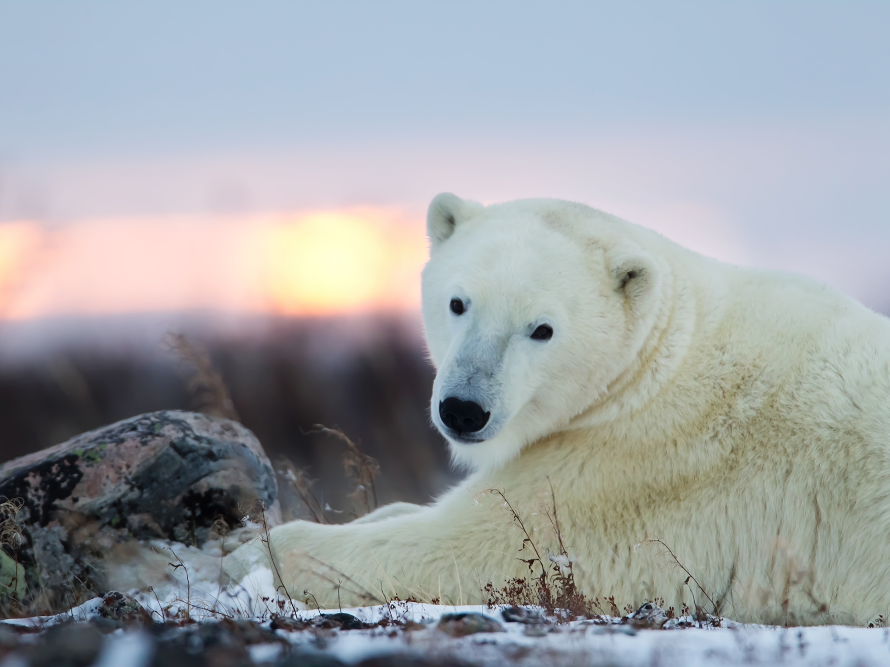
Polar bears are trying to adapt to a warming Arctic. It’s not working.

• Perpetual Planet
• Environment
• History & Culture
• Paid Content

History & Culture

• Mind, Body, Wonder
• Terms of Use
• Privacy Policy
• Your US State Privacy Rights
• Children's Online Privacy Policy
• Interest-Based Ads
• About Nielsen Measurement
• Do Not Sell or Share My Personal Information
• Nat Geo Home
• Attend a Live Event
• Book a Trip
• Inspire Your Kids
• Shop Nat Geo
• Visit the D.C. Museum
• Learn About Our Impact
• Support Our Mission
• Advertise With Us
• Customer Service
• Renew Subscription
• Manage Your Subscription
• Work at Nat Geo
• Sign Up for Our Newsletters
• Contribute to Protect the Planet

Copyright © 1996-2015 National Geographic Society Copyright © 2015-2024 National Geographic Partners, LLC. All rights reserved

• Open supplemental data
• Reference Manager
• Simple TEXT file

People also looked at

Original research article, the unseen effects of deforestation: biophysical effects on climate.

• 1 Department of Environmental Sciences, University of Virginia, Charlottesville, VA, United States
• 2 The Woodwell Climate Research Center, Falmouth, MA, United States
• 3 The Alliance of Bioversity International and the International Center for Tropical Agriculture, Cali, Colombia

Climate policy has thus far focused solely on carbon stocks and sequestration to evaluate the potential of forests to mitigate global warming. These factors are used to assess the impacts of different drivers of deforestation and forest degradation as well as alternative forest management. However, when forest cover, structure and composition change, shifts in biophysical processes (the water and energy balances) may enhance or diminish the climate effects of carbon released from forest aboveground biomass. The net climate impact of carbon effects and biophysical effects determines outcomes for forest and agricultural species as well as the humans who depend on them. Evaluating the net impact is complicated by the disparate spatio-temporal scales at which they operate. Here we review the biophysical mechanisms by which forests influence climate and synthesize recent work on the biophysical climate forcing of forests across latitudes. We then combine published data on the biophysical effects of deforestation on climate by latitude with a new analysis of the climate impact of the CO 2 in forest aboveground biomass by latitude to quantitatively assess how these processes combine to shape local and global climate. We find that tropical deforestation leads to strong net global warming as a result of both CO 2 and biophysical effects. From the tropics to a point between 30°N and 40°N, biophysical cooling by standing forests is both local and global, adding to the global cooling effect of CO 2 sequestered by forests. In the mid-latitudes up to 50°N, deforestation leads to modest net global warming as warming from released forest carbon outweighs a small opposing biophysical cooling. Beyond 50°N large scale deforestation leads to a net global cooling due to the dominance of biophysical processes (particularly increased albedo) over warming from CO 2 released. Locally at all latitudes, forest biophysical impacts far outweigh CO 2 effects, promoting local climate stability by reducing extreme temperatures in all seasons and times of day. The importance of forests for both global climate change mitigation and local adaptation by human and non-human species is not adequately captured by current carbon-centric metrics, particularly in the context of future climate warming.

Introduction

Failure to stabilize climate is in itself a large threat to biodiversity already at risk from deforestation. Protection, expansion, and improved management of the world’s forests represent some of the most promising natural solutions to the problem of keeping global warming below 1.5–2 degrees ( Griscom et al., 2017 ; Roe et al., 2019 ). Forests sequester large quantities of carbon; of the 450–650 Pg of carbon stored in vegetation ( IPCC, 2013 ), over 360 Pg is in forest vegetation ( Pan et al., 2013 ). Adding the carbon in soils, forests contain over 800 PgC, almost as much as is currently stored in the atmosphere ( Pan et al., 2013 ). In addition, forests are responsible for much of the carbon removal by terrestrial ecosystems which together remove 29% of annual CO 2 emissions (∼11.5 PgC; Friedlingstein et al., 2019 ). Globally, forest loss not only releases a large amount of carbon to the atmosphere, but it also significantly diminishes a major pathway for carbon removal long into the future ( Houghton and Nassikas, 2018 ). Tropical forests, which hold the greatest amount of aboveground biomass and have one of the fastest carbon sequestration rates per unit land area ( Harris et al., 2021 ), face the greatest deforestation pressure ( FAO, 2020 ). Given the long half-life and homogenous nature of atmospheric CO 2 , current forest management decisions will have an enduring impact on global climate through effects on CO 2 alone. However, forests also impact climate directly through controls on three main biophysical mechanisms: albedo, evapotranspiration (ET) and canopy roughness.

The direct biophysical effects of forests moderate local climate conditions. As a result of relatively low albedo, forests absorb a larger fraction of incoming sunlight than brighter surfaces such as bare soil, agricultural fields, or snow. Changes in albedo can impact the radiation balance at the top of the atmosphere and thus global temperature. The local climate, however, is not only impacted by albedo changes but also by how forests partition incoming solar radiation between latent and sensible heat. Deep roots and high leaf area make forests very efficient at moving water from the land surface to the atmosphere via ET, producing latent heat. Thus, beneath the forest canopy, the sensible heat flux and associated surface temperature are relatively low, especially during the growing season when ET is high ( Davin and de Noblet-Ducoudré, 2010 ; Mildrexler et al., 2011 ; Alkama and Cescatti, 2016 ). This cooling is enhanced by the relatively high roughness of the canopy, which strengthens vertical mixing and draws heat and water vapor away from the surface. Higher in the atmosphere, as water vapor condenses, the latent heat is converted to sensible heat. As a result, warming that began with sunlight striking the canopy is felt higher in the atmosphere rather than in the air near the land surface. These non-radiative processes stabilize local climate by reducing both the diurnal temperature range and seasonal temperature extremes ( Lee et al., 2011 ; Zhang et al., 2014 ; Alkama and Cescatti, 2016 ; Findell et al., 2017 ; Forzieri et al., 2017 ; Hirsch et al., 2018 ; Lejeune et al., 2018 ). Their impact on global climate, however, is less clear.

Despite high spatial variability, forest biophysical impacts do follow predictable latitudinal patterns. In the tropics, higher incoming solar radiation and moisture availability provide more energy to drive ET and convection, which in combination with roughness overcome the warming effect of low albedo, and result in year round cooling by forests. At higher latitudes, where incoming solar radiation is highly seasonal, the impacts of ET and surface roughness are diminished ( Anderson et al., 2011 ; Li et al., 2015 ) and albedo is the dominant biophysical determinant of the climate response. In boreal forests, relatively low albedo and low ET cause strong winter and spring warming. In the summer, higher incoming radiation and somewhat higher ET result in mild cooling by boreal forests ( Alkama and Cescatti, 2016 ). In the mid-latitudes, forest cover results in mild biophysical evaporative cooling in the summer months and mild albedo warming in the winter months ( Davin and de Noblet-Ducoudré, 2010 ; Li et al., 2015 ; Schultz et al., 2017 ). The latitude of zero net biophysical effect, the point at which the annual effect of the forest shifts from local cooling to local warming, ranges from 30 to 56°N in the literature ( Figure 1 ). These generalized latitudinal trends can be modified by aridity, elevation, species composition, and other characteristics, which vary across a range of spatial scales ( Anderson-Teixeira et al., 2012 ; Williams et al., 2021 ).

Figure 1. Latitude of net zero biophysical effect of forests on local temperature varies from 30 to 56°N. Above the line, forest cover causes local warming; below the line, forest cover causes local cooling. The thickness of the line indicates the number of studies that show forest cooling up to that threshold. Data sources as indicated.

Various mechanisms can amplify or dampen a forest’s direct effects on the energy and water balance, with climate impacts in the immediate vicinity, in remote locations, or both ( Bonan, 2008 ). Indirect biophysical effects are particularly important in the boreal region where snow-forest albedo interactions are prevalent. Low albedo forests typically mask high albedo snow, resulting in local radiative warming ( Jiao et al., 2017 ). At the larger scale this forest-induced warming is transferred to the oceans and further amplified by interactions with sea ice ( Brovkin et al., 2004 ; Bala et al., 2007 ; Davin and de Noblet-Ducoudré, 2010 ; Laguë and Swann, 2016 ). In fact, indirect biophysical feedbacks appear to dominate the global temperature response to deforestation in the boreal region ( Devaraju et al., 2018 ). Future climate warming may alter the strength of such feedbacks, depending on the rate at which forests expand northward and the extent and persistence of spring snow cover in a warmer world.

In the tropics, where ET and roughness are the dominant biophysical drivers, forests cool the lower atmosphere, but also provide the water vapor to support cloud formation ( Teuling et al., 2017 ). Clouds whiten the atmosphere over forests and thus increase albedo, at least partially offsetting the inherently low albedo of the forest below ( Heald and Spracklen, 2015 ; Fisher et al., 2017 ). However, the water vapor in clouds also absorbs and re-radiates heat, counteracting some of the cloud albedo-induced cooling ( Swann et al., 2012 ). In the Amazon basin, evidence suggests that deep clouds may occur more frequently over forested areas as a result of greater humidity and consequently greater convective available potential energy ( Wang et al., 2009 ). The impact of tropical deforestation on cloud formation is modified by biomass burning aerosols ( Liu et al., 2020 ) and the net impact on global climate is unclear. Quantifying these indirect biophysical feedback effects is an ongoing challenge for the modeling community particularly in the context of constraining future climate scenarios.

Forest production of biogenic volatile organic compounds (BVOC), which affect both biogeochemical and biophysical processes, further complicate quantification of the net climate impact of forests. BVOC and their oxidation products regulate secondary organic aerosols (SOA), which are highly reflective and result in biophysical cooling. SOA also act as cloud condensation nuclei, enhancing droplet concentrations and thereby increasing cloud albedo, which leads to additional biophysical cooling ( Topping et al., 2013 ). On the other hand, SOA can also cause latent heat release in deep convective cloud systems resulting in strong radiative warming of the atmosphere ( Fan et al., 2012 , 2013 ). Furthermore, through impacts on the oxidative capacity of the atmosphere, BVOC increase the lifetime of methane and lead to the formation of tropospheric ozone in the presence of nitrogen oxides ( Arneth et al., 2011 ; McFiggans et al., 2019 ). The persistence of ozone and methane (both greenhouse gases) results in a biogeochemical warming effect. The net effect of forest BVOC at both local and global scales remains uncertain. Current evidence, from modeling forest loss since 1850, suggests that BVOC result in a small net cooling, if indirect cloud effects are included ( Scott et al., 2018 ). The strongest effect is in the tropics, where BVOC production is highest ( Messina et al., 2016 ).

An improved understanding of the combined effects of forest carbon and biophysical controls on both local and global climate is necessary to guide policy decisions that support global climate mitigation, local adaptation and biodiversity conservation. The relative importance of forest carbon storage and biophysical effects on climate depend in large part on the spatial and temporal scale of interest. Local surface or air temperature may not be sensitive to the incremental impact of atmospheric CO 2 removed by forests growing in a particular landscape or watershed. In contrast, local temperature is sensitive to biophysical changes in albedo, ET and roughness. At regional and global scales, where the cumulative effects of forests on atmospheric CO 2 become apparent in the temperature response, we can usefully compare these impacts. Estimates of the relative impact of biophysical and biogeochemical (e.g., carbon cycle) processes on global or zonal climate have been provided primarily by model simulations of large-scale deforestation or afforestation ( Table 1 ). These studies generally show that CO 2 effects on global temperature are many times greater than the biophysical effects of forest cover or forest loss. In models depicting global or zonal deforestation outside the tropics, however, global warming from CO 2 release offsets only 10–90% of the global biophysical cooling. The global CO 2 effects of total deforestation in the tropics greatly outweigh the global biophysical effects ( Table 1 ). With the exception of Davin and de Noblet-Ducoudré (2010) , these studies have estimated the net contribution of biophysical processes, without isolating the individual biophysical components. Here, we provide a new analysis of CO 2 -induced warming from deforestation by 10° latitudinal increments ( Supplementary Information 1 ). We then compare the CO 2 effect with the only published determination of biophysical effects by latitude ( Davin and de Noblet-Ducoudré, 2010) to clarify the potential net impact of forest loss in a particular region on local and global climate.

Table 1. Forest effects on global temperature in modeling experiments from biogeochemical (CO 2 ) versus biophysical impacts (albedo, evapotranspiration and roughness as well as changes in atmospheric and ocean circulation, snow and ice, and clouds).

Materials and Methods

In the scientific literature, biophysical impacts have been quantified using a number of different methods. In situ observational data, including weather station and eddy flux measurements, have shaped our understanding of the direct biophysical impacts of forests on the surface energy balance. With the advantage of high temporal resolution, they allow for process level investigation of forest biophysical impacts and attribution of temperature changes to particular biophysical forcings, both radiative (albedo) and non-radiative (ET and roughness) ( Lee et al., 2011 ; Luyssaert et al., 2014 ; Vanden Broucke et al., 2015 ; Bright et al., 2017 ; Liao et al., 2018 ). Remote sensing techniques have recently been used to extrapolate to larger scales, providing a global map of forest cover effects on local climate ( Li et al., 2015 ; Alkama and Cescatti, 2016 ; Bright et al., 2017 ; Duveiller et al., 2018 ; Prevedello et al., 2019 ). However, in contrast to in situ approaches which generally measure near surface air temperature (generally but not always at 2 m), remote sensing studies have investigated the response of land surface temperature (i.e., skin temperature) which is 0.5–3 times more sensitive to forest cover change ( Alkama and Cescatti, 2016 ; Novick and Katul, 2020 ).

Generally, both in situ and remote sensing analyses have adopted a space-for-time approach where differences in surface climate of neighboring forest and non-forest sites are used as proxies for the climate signal from deforestation/afforestation over time. This approach assumes that neighboring sites share a common background climate and that any temperature differences between them can be attributed solely to differences in forest cover. Consequently, large-scale biophysical feedback effects are ignored. New observation-based methodologies have been devised to investigate impacts from ongoing land use change rather than estimating climate sensitivities to idealized forest change ( Alkama and Cescatti, 2016 ; Bright et al., 2017 ; Prevedello et al., 2019 ), however, they too measure only local biophysical impacts.

Numerical modeling of paired climate simulations with contrasting forest cover is necessary to investigate the net climate response to forest cover change, including both local and non-local impacts. Model simulations have focused on idealized scenarios of large-scale deforestation/afforestation which are more likely to trigger large-scale climate feedbacks than more realistic incremental forest cover change. Discrepancies between observed and modeled results may be due in part to the influence of indirect climate feedbacks that are not captured by observations ( Winckler et al., 2017a , 2019a ; Chen and Dirmeyer, 2020 ). Unfortunately, model resolution is currently too coarse to guide local policy decisions. Modeling results are also plagued by a number of uncertainties associated with the partitioning of energy between latent or sensible heat ( de Noblet-Ducoudré et al., 2012 ). The predicted impacts of similar land cover changes are model specific and can vary in sign, magnitude, and geographical distribution ( Devaraju et al., 2015 ; Lawrence and Vandecar, 2015 ; Garcia et al., 2016 ; Laguë and Swann, 2016 ; Stark et al., 2016 ; Quesada et al., 2017 ; Boysen et al., 2020 ) and therefore must be viewed with caution. In this paper, we synthesize all types of observational data from the literature to illustrate the biophysical impacts of forests on local climate. However, given that local impacts have been extensively explored and summarized in the past ( Anderson et al., 2011 ; Perugini et al., 2017 ), and because we wish to include indirect effects and feedbacks, we rely predominantly on modeling studies and our own calculations to elucidate the role of forests at different latitudes in shaping climate.

Effects on Global Temperature From Deforestation by 10° Latitude Band

We combined published data on biophysical effects of deforestation by latitude with our own analysis of CO 2 effects from deforestation by latitude to compare the relative strength of biophysical factors and CO 2 (the dominant biogeochemical factor) affecting global climate. Most modeling experiments available in the literature involve total deforestation at all latitudes, and the ocean feedbacks prove very strong ( Davin and de Noblet-Ducoudré, 2010) . Here, we consider land-only effects within a given 10° latitudinal band as this scale of impact is more indicative of the effects of regional or more incremental change on global temperature than the combined land/ocean effects. Finer scale, more realistic forest loss scenarios would not trigger massive cooling through albedo effects on the oceans. Area-scaled, land-only biophysical effects from deforestation provide the most realistic comparison with the effects of carbon stored by forests, and released through deforestation, at a given latitude. The biophysical response was derived from the results of Davin and de Noblet-Ducoudré (2010) who simulated total deforestation and decomposed the temperature response, by 10° latitude bands, into the fraction due to albedo, evapotranspiration, roughness and a non-linear response (see Supplementary Table 1 ).

The biogeochemical response was estimated by accounting for the CO 2 effect of deforestation, using existing biomass data and known equilibrium temperature sensitivity to doubled CO 2 . The principal input to our analysis is a 2016 global extension of the 500-m resolution aboveground carbon density (ACD) change (2003–2016) product applied by Walker et al. (2020) to the Amazon basin. It is based on an approach to pantropical ACD change estimation developed by Baccini et al. (2017) . The pantropical product combined field measurements with colocated NASA ICESat GLAS spaceborne light detection and ranging (LiDAR) data to calibrate a machine-learning algorithm that produced estimates of ACD using MODIS satellite imagery. This approach was modified for application to the extratropics, principally the temperate and boreal zones but also extratropical South America, Africa and Australia, using 47 allometric equations compiled from 27 unique literature sources for relating field-based measurements of aboveground biomass to airborne LiDAR metrics ( Chapman et al., 2020 ). These equations were used to predict ACD within the footprints of GLAS LiDAR acquisitions in each region with the result being a pseudo-inventory of LiDAR-based estimates of ACD spanning the extratropics. This dataset was then combined with the pantropical dataset first generated by Baccini et al. (2012) to produce a global database of millions of spatially explicit ACD predictions. This database was used to calibrate six ecoregional MODIS-based models for the purposes of generating a global 500-m resolution map of ACD for the year 2016. Additional details on these methods can be found in Chapman et al. (2020) .

The total aboveground carbon (GtC) was summed for each 10° latitude band and converted to CO 2 (GtC*44/12 = GtCO 2 , Supplementary Information 1 ). The mass of CO 2 was converted to ppm CO 2 in the atmosphere (2.12 Gt/ppm). The derived CO 2 concentration was reduced by 23% to account for ocean uptake ( Global Carbon Project, 2019 ). We assumed that no uptake occurred on land, as the carbon stock in vegetation was completely removed in our experiment to match what occurred in Davin and de Noblet-Ducoudré (2010) . Next, we calculated the global temperature response to the increase in atmospheric CO 2 due to the CO 2 released by completely deforesting each 10° latitudinal band using the equilibrium temperature sensitivity derived from general circulation models. Given the accepted value of 3°C (±1.5°C) for a doubling of atmospheric CO 2 (an increase of 280 ppm) (IPCC, 2013), we determined that temperature sensitivity is equivalent to 0.107°C (±0.054°C) for every 10 ppm increase in atmospheric CO 2 content.

To determine the global temperature response to deforestation of a given band, we calculated the area-weighted values for each biophysical response within each latitude band. The area encompassed by 10° of latitude increases toward the equator. Thus, to determine the contribution of a given band to a global temperature response, scaling by the surface area within the band was essential. We used average temperature responses over the land only to avoid the strong bias associated with ocean feedbacks from global scale implementation of deforestation.

For the global analysis, we also determined the contribution of BVOC to global temperature change for deforestation of each 10° of latitude. Scott et al. (2018) described the warming from deforestation due to BVOC in relation to the amount of cooling due to changes in albedo. For the tropics, the BVOC effect on global temperature was 17% of the albedo effect. For the temperate zone, it was 18% and for the boreal, it was 2% of the albedo effect. We applied these scalars (with an opposite sign) to the albedo figures for each 10° latitude band.

Effects on Regional (Local) Temperature From Deforestation by 10° Latitude Band

To analyze the effect of deforesting 10° of latitude on the temperature within that latitude zone (‘local’ effect), we did not scale by area within the band. Rather we assessed the average temperature change across the band, locally felt, as reported in the original study. The CO 2 effect was calculated as above and then scaled to reflect the sensitivity of a given latitudinal band to a global forcing. Only the CO 2 emitted by the latitudinal band itself was considered when determining the locally felt effects of CO 2 in a given band. Our experimental design involved global deforestation and all emitted CO 2 would have had an effect in a given band, but the point of the analysis was to isolate the temperature change caused by forests in a given latitude. We determined the latitudinal sensitivity to warming in response to added CO 2 from a re-analysis of global 2 m temperature data (CERA-20C) obtained from the European Centre for Medium-Range Weather https://www.ecmwf.int/en/forecasts/datasets/reanalysis-datasets/cera-20c . We compared average temperatures from 1901 to 1910 and 2001–2010, by latitude on land only (inadequate land only data for 50–60S and 80–90N; for those, we do not report a locally felt CO 2 effect). Then we divided the temperature change for each latitude band by the change in global temperature over the same period. We scaled the effect of CO 2 emitted by a given 10° latitude band by this sensitivity to represent the influence of non-linear responses such as polar amplification (see Supplementary Information 1 and Supplementary Table 2 ).

Biophysical Effects of Deforestation on Local Climate: A Broader Context

Our analysis is the first to compare regional scale biophysical and CO 2 impacts from regional scale deforestation but the literature is replete with data on local biophysical impacts. The results for local biophysical effects (100s of m to 100s of km) agree with our results at the regional scale (below). Figures 2 , 3 synthesize local biophysically-driven temperature responses to deforestation, as indicated by forest/no-forest comparisons or forest change over time, from the scientific literature. Satellite and flux tower data indicate that surface temperatures in tropical forests are significantly lower than in cleared areas nearby. On an annual basis, local surface cooling of 0.2–2.4°C has been observed (mean 0.96°C, Figure 2 and Supplementary Information 2 ). In the temperate zone, satellite studies of land surface temperature (which is more sensitive than the temperature of the air at 2 m) have shown biophysical cooling from forest cover, or biophysical warming from deforestation (0.02–1.0°C, mean of 0.4°C; see Figure 2 and Supplementary Information 2 ). Both in situ and satellite data generally indicate an average annual cooling of under 1°C from boreal deforestation ( Figure 2 ). Across latitudinal zones, warming from deforestation is generally greater during the day, and during the dry (hot) season ( Figure 3 ).

Figure 2. Local average annual temperature change in response to deforestation (black symbols) or afforestation (green symbols) as determined by comparing neighboring forested and open land (space for time approach) or measuring forest change over time in the tropics, temperate and boreal zones, by (A) in situ or (B) satellite based land surface temperature measurements (0 m, triangles) or air temperature measurements (2 m, circles). See Supplementary Information 2 for data sources.

Figure 3. Local temperature change in response to deforestation by season and time of day in the various climate zones as determined by comparing neighboring forested and open land (space for time approach) or measuring forest change over time. Warm/dry season response, averaged over the entire diurnal cycle, in red shading and cold/wet season response in blue shading. Daytime response, averaged over the entire annual cycle, in yellow shading and nighttime response in gray shading. See Supplementary Information 3 for data sources.

CO 2 -Induced Warming Versus Biophysical Effects on Regional (Local) Temperature From Deforestation by 10° Latitude Band

As expected, the regionally felt effect of regionally (10° band) produced CO 2 is very small compared to any individual biophysical effect or the sum of all non-CO 2 effects ( Figure 4 ). These results indicate that the net impact of all non-CO 2 effects is negligible between 20 and 30N. Beyond 30N the local biophysical response to deforestation is cooling. In the broader literature, this latitude of net zero biophysical effect on local temperature is generally between 30 and 40N ( Figure 1 ).

Figure 4. Effect of complete deforestation on local annual temperature by climate factor, averaged across the land surface within a 10° latitudinal band. Complete deforestation was implemented globally and analyzed by 10° latitudinal bands ( Davin and de Noblet-Ducoudré, 2010) . The CO 2 effect was determined from total aboveground biomass in each 10° band after Walker et al. (2020) and scaled by CERA-derived sensitivity by latitude. Inset distinguishes the sum of all local biophysical effects from local CO 2 effects.

Biophysical Effects on Global Temperature From Deforestation by 10° Latitude Band

For most latitudinal bands, the strongest biophysical effect of deforestation is cooling from albedo changes. In the tropics, however, the warming effect of lost roughness is comparable to or greater than the albedo effect ( Figure 5A ). Adding the warming from lost evapotranspiration, the net biophysical effect from tropical deforestation is global warming, as much as 0.1°C contributed each by latitudes 0°–10°S and 0°–10°N. The net biophysical effect of intact tropical forest, therefore, is global cooling; slightly more cooling if BVOCs are also considered (see Figure 5B ). Roughness effects are generally greater than evapotranspiration effects across latitudes providing a strong counterbalance to albedo effects ( Davin and de Noblet-Ducoudré, 2010 ; Burakowski et al., 2018 ; Winckler et al., 2019b ; Figure 5A ). Albedo almost balances the combined effect of roughness, evapotranspiration, BVOC and non-linear effects between 20 and 30°N resulting in close to zero net biophysical effect on global temperature ( Figure 5B ). From 30–40°N and northward, albedo dominates, and the net biophysical effect of deforestation is cooling.

Figure 5. Effect of complete deforestation on global temperature by 10° band of latitude. (A) Contribution to global temperature change by climate forcing factor. Biophysical factors are from Davin and de Noblet-Ducoudré, 2010 , area-weighted. BVOC effects are estimated relative to albedo effects based on Scott et al., 2018 . CO 2 effect is based on aboveground live biomass for each 10° latitudinal band following Baccini et al., 2017 and Walker et al., 2020 . (B) Net biophysical and BVOC effect versus CO 2 effect. (C) Cooling or warming effects of deforestation by 10° latitudinal band (BVOC included). “Forests as mountains” map of aboveground biomass carbon in woody vegetation ca. 2016 courtesy of Woodwell Climate Research Center and shaded to indicate where deforestation results in net global warming. See Supplementary Information 1 for details.

CO 2 -Induced Warming Versus Biophysical Effects on Global Temperature From Deforestation by 10° Latitude Band

From 30°S to 30°N, the biophysical effect of deforesting a given 10° latitudinal band is about half as great and in the same direction as the CO 2 effect: global warming. Biophysical warming is around 60% as great as warming from released CO 2 in the outer tropics (20°S–10°S and 10°N–20°N) and about 35% as great in the heart of the tropics (10°S–10°N). Biophysical cooling due to deforestation from 30°N to 40°N offsets about 40% of the warming associated with carbon loss from deforestation; from 40°N to 50°N biophysical effects offset 85% of CO 2 effects ( Figure 5B ). Above 50°N, biophysical global cooling is 3–6 times as great as CO 2 induced global warming. The net impact of deforestation (effects of CO 2 , biophysical processes and BVOC combined) is warming at all latitudes up to 50N ( Figure 5C ). Thus, from 50S to 50N, an area that encompasses approximately 65% of global forests ( FAO, 2020 ), deforestation results in global warming ( Figure 5C ).

All Forests Provide Local Climate Benefits Through Biophysical Effects

Ignoring biophysical effects on local climate means casting aside a powerful inducement to promote global climate goals and advance forest conservation: local self-interest. The biogeochemical effect of forests tends to dominate the biophysical effect at the global scale because physical effects in one region can cancel out effects in another. Nevertheless, biophysical effects are very important, and can be very large, at the local scale (e.g., Anderson-Teixeira et al., 2012 ; Bright et al., 2015 ; Jiao et al., 2017 ; Figures 2 – 4 ). The role of forests in maintaining critical habitat for biodiversity is well known, but new research on extinction confirms the role of forests in maintaining critical climates to support biodiversity. Changes in maximum temperature are driving extinction, not changes in average temperature ( Román-Palacios and Wiens, 2020 ). Deforestation is associated with an increase in the maximum daily temperature throughout the year in the tropics and during the summer in higher latitudes ( Lee et al., 2011 ; Zhang et al., 2014 ). Of course deforestation also increases average daytime temperatures in boreal, mid-latitude and tropical forests ( Figure 3 ). The biophysical effects of forests also moderate local and regional temperature extremes such that extremely hot days are significantly more common following deforestation even in the mid- and high latitudes ( Vogel et al., 2017 ; Stoy, 2018 ). Historical deforestation explains ∼1/3 of the present day increase in the intensity of the hottest days of the year at a given location ( Lejeune et al., 2018 ). It has also increased the frequency and intensity of hot dry summers two to four fold ( Findell et al., 2017 ). Local increases in extreme temperatures due to forest loss are of comparable magnitude to changes caused by 0.5°C of global warming ( Seneviratne et al., 2018 ). Forests provide local cooling during the hottest times of the year anywhere on the planet, improving the resilience of cities, agriculture, and conservation areas. Forests are critical for adapting to a warmer world.

Forests also minimize risks due to drought associated with heat extremes. Deep roots, high water use efficiency, and high surface roughness allow trees to continue transpiring during drought conditions and thus to dissipate heat and convey moisture to the atmosphere. In addition to this direct cooling, forest ET can influence cloud formation ( Stoy, 2018 ), enhancing albedo and potentially promoting rainfall. The production of BVOCs and organic aerosols by forests accelerates with increasing temperatures, enhancing direct or indirect (cloud formation) albedo effects. This negative feedback on temperature has been observed to counter anomalous heat events in the mid-latitudes ( Paasonen et al., 2013 ).

Some Forests Provide Global Climate Benefits Through Biophysical Effects

Disregarding the biophysical effects of specific forests on global climate means under-selling some forest actions and over-selling others. The response to local forest change is not equivalent for similar sized areas in different latitudes. According to Arora and Montenegro (2011) warming reductions per unit reforested area are three times greater in the tropics than in the boreal and northern temperate zone due to a faster carbon sequestration rate magnified by year-round biophysical cooling. Thus, considering biophysical effects significantly enhances both the local and global climate benefits of land-based mitigation projects in the tropics (see Figures 4 , 5 ).

Constraints on Forest Climate Benefits in the Future

Climate change is likely to alter the biophysical effect of forests in a variety of ways. Deforestation in a future (warmer) climate could warm the tropical surface 25% more than deforestation in a present-day climate due to stronger decreases in turbulent heat fluxes ( Winckler et al., 2017b ). In a warmer climate, reduced snow cover in the temperate and boreal regions will lead to a smaller albedo effect and thus less biophysical cooling with high latitude deforestation. In addition to snow cover change, future rainfall regimes will affect the response of climate to changes in forest cover ( Pitman et al., 2011 ) as rainfall limits the supply of moisture available for evaporative cooling. Increases in water use efficiency due to increasing atmospheric CO 2 may reduce evapotranspiration ( Keenan et al., 2013 ), potentially reducing the local cooling effect of forests and altering atmospheric moisture content and dynamics at local to global scales. Future BVOC production may increase due to warming and simultaneously decline due to CO 2 suppression ( Lathière et al., 2010 ; Unger, 2014 ; Hantson et al., 2017 ). The physiological and ecological responses of forests to warming, rising atmospheric CO 2 and changing precipitation contribute to uncertainty in the biophysical effect of future forests on climate.

Forest persistence is essential for maintaining the global benefits of carbon removals from the atmosphere and the local and global benefits of the physical processes described above. Changing disturbance regimes may limit forest growth and regrowth in many parts of the world. Dynamic global vegetation models currently show an increasing terrestrial carbon sink in the future. This sink is thought to be due to the effects of fertilization by rising atmospheric CO 2 and N deposition on plant growth as well as the effects of climate change lengthening the growing season in northern temperate and boreal areas ( Le Quéré et al., 2018 ). Free-air carbon dioxide enrichment (FACE) experiments often show increases in biomass accumulation under high CO 2 but results are highly variable due to nutrient limitations and climatic factors ( Feng et al., 2015 ; Paschalis et al., 2017 ; Terrer et al., 2018 ). Climate change effects on the frequency and intensity of pest outbreaks are poorly studied, but are likely to be significant, particularly at the margins of host ranges. Warmer springs and winters are already increasing insect-related tree mortality in boreal forests through increased stress on the tree hosts and direct effects on insect populations ( Volney and Fleming, 2000 ; Price et al., 2013 ).

Climate also affects fire regimes. In the tropics, fire regimes often follow El Niño cycles ( van der Werf et al., 2017 ). As temperatures increase, however, fire and rainfall are decoupled as the flammability of forests increases even in normal rainfall years ( Fernandes et al., 2017 ; Brando et al., 2019 ). Fire frequency is also increasing in some temperate and boreal forests, with a discernable climate change signal ( Abatzoglou and Williams, 2016 ). Modeling exercises indicate that this trend is expected to continue with increasing damage to forests as temperatures rise and fire intensity increases ( De Groot et al., 2013 ).

In addition to changes induced by warming, continued deforestation could severely stress remaining forests by warming and drying local and regional climates ( Lawrence and Vandecar, 2015 ; Costa et al., 2019 ; Gatti et al., 2021 ). In the tropics, a tipping point may occur, potentially resulting in a shift to shorter, more savannah-like vegetation and altering the impact of vast, previously forested areas on global climate ( Nobre et al., 2016 ; Brando et al., 2019 ). Some of these processes are included in climate models and some are not. The gaps leave considerable uncertainty. Nevertheless, a combination of observations, models, and theory gives us a solid understanding of the biophysical effects of forests on climate at local, regional and global scales. We can use that knowledge to plan forest-based climate mitigation and adaptation.

Mitigation Potential of Forests: Byond the Carbon/Biophysical Divide

If instead of focusing on the contrast between biophysical and biochemical impacts of forests and forest loss, we focus on the potential of forests to cool the planet through both pathways, another picture emerges. By our conservative estimate, through the combined effects on CO 2 , BVOC, roughness and evapotranspiration, forests up to 50°N provide a net global cooling that is enough to offset warming associated with their low albedo. Given the most realistic pathways of forest change in the future (not complete deforestation of a 10° latitudinal band, or an entire biome), global climate stabilization benefits likely extend beyond 50°N. For the 29% of the global land surface that lies beyond 50°N, forests may warm the planet, but only as inferred from assessing the effects of complete zonal deforestation with all the associated, and powerful, land-ocean feedbacks spawned by largescale forest change in the boreal zone. Forests above 50°N, like forests everywhere, provide essential local climate stabilization benefits by reducing surface temperatures during the warm season as well as periods of extreme heat or drought. Indeed, they also reduce extreme cold.

Creating a fair and effective global arena for market-based solutions to climate change requires attention to all the ways that forests affect climate, including the biophysical effects. Future metrics of forest climate impacts should consider the effects of deforestation beyond CO 2 . Only recently have modelers begun to include BVOC. Doing so means that the albedo of intact forests (or the atmosphere above them) is higher due to the creation of SOA and subsequent cloud formation. Modeled deforestation thus results in less of a change in albedo, reducing the biophysical cooling effect. Similarly, accounting for the ozone and methane effects of BVOC reduces the biogeochemical warming from deforestation ( Scott et al., 2018 ). In addition, especially in the tropics, deforestation reduces the strength of the soil CH 4 sink ( Dutaur and Verchot, 2007 ). While a small change relative to the atmospheric pool of CH 4 (the second most important greenhouse gas), the loss of this sink is equivalent to approximately 13% of the current rate of increase in atmospheric CH 4 ( Saunois et al., 2016 ). We already have the data ( Figure 5 ) to begin conceptualizing measures to coarsely scale CO 2 impacts of forest change by latitude. Finer resolution of latitude, background climate (current and future) and forest type would improve any such new, qualifying metric for the climate mitigation value of forests.

The role of forests in addressing climate change extends beyond the traditional concept of CO 2 mitigation which neglects the local climate regulation services they provide. The biophysical effects of forest cover can contribute significantly to solving local adaptation challenges, such as extreme heat and flooding, at any latitude. The carbon benefits of forests at any latitude contribute meaningfully to global climate mitigation. In the tropics, however, where forest carbon stocks and sequestration rates are highest, the biophysical effects of forests amplify the carbon benefits, thus underscoring the critical importance of protecting, expanding, and improving the management of tropical forests. Perhaps it is time to think more broadly about what constitutes global climate mitigation. If climate mitigation means limiting global warming, then clearly the biophysical effects of deforestation must be considered in addition to its effects on atmospheric CO 2 . We may further consider whether mitigation is too narrow a scope for considering the climate benefits provided by forests. Climate policy often separates mitigation from adaptation, but the benefits of forests clearly extend into both realms.

Data Availability Statement

The original contributions presented in the study are included in the article/ Supplementary Material , further inquiries can be directed to the corresponding author.

Author Contributions

DL conceived the presented idea. All authors helped perform the computations, discussed the results, and contributed to the final manuscript.

Financial support from the University of Virginia and the Climate and Land Use Alliance grant #G-1810-55876.

Conflict of Interest

The authors declare that the research was conducted in the absence of any commercial or financial relationships that could be construed as a potential conflict of interest.

Publisher’s Note

All claims expressed in this article are solely those of the authors and do not necessarily represent those of their affiliated organizations, or those of the publisher, the editors and the reviewers. Any product that may be evaluated in this article, or claim that may be made by its manufacturer, is not guaranteed or endorsed by the publisher.

Acknowledgments

Thanks to Frances Seymour, Michael Wolosin, Billie L. Turner, Ruth DeFries, and the reviewers for feedback on this manuscript and to the University of Virginia and the Climate and Land Use Alliance grant #G-1810-55876 for financial support.

Supplementary Material

The Supplementary Material for this article can be found online at: https://www.frontiersin.org/articles/10.3389/ffgc.2022.756115/full#supplementary-material

Abatzoglou, J. T., and Williams, A. P. (2016). Impact of anthropogenic climate change on wildfire across western US forests. Proc. Natl. Acad. Sci. U.S.A. 113, 11770–11775. doi: 10.1073/pnas.1607171113

PubMed Abstract | CrossRef Full Text | Google Scholar

Alkama, R., and Cescatti, A. (2016). Biophysical climate impacts of recent changes in global forest cover. Science 351, 600–604. doi: 10.1126/science.aac8083

Anderson, R. G., Canadell, J. G., Randerson, J. T., Jackson, R. B., Hungate, B. A., Baldocchi, D. D., et al. (2011). Biophysical considerations in forestry for climate protection. Front. Ecol. Environ. 9, 174–182. doi: 10.1890/090179

CrossRef Full Text | Google Scholar

Anderson-Teixeira, K. J., Snyder, P. K., Twine, T. E., Cuadra, S. V., Costa, M. H., and DeLucia, E. H. (2012). Climate-regulation services of natural and agricultural ecoregions of the Americas. Nat. Clim. Change 2:177. doi: 10.1038/nclimate1346

Arneth, A., Schurgers, G., Lathiere, J., Duhl, T., Beerling, D. J., Hewitt, C. N., et al. (2011). Global terrestrial isoprene emission models: sensitivity to variability in climate and vegetation. Atmos. Chem. Phys. 11, 8037–8052. doi: 10.1002/2013JD021238

Arora, V. K., and Montenegro, A. (2011). Small temperature benefits provided by realistic afforestation efforts. Nat. Geosci. 4, 514–518. doi: 10.1038/ngeo1182

Baccini, A. G. S. J., Goetz, S. J., Walker, W. S., Laporte, N. T., Sun, M., Sulla-Menashe, D., et al. (2012). Estimated carbon dioxide emissions from tropical deforestation improved by carbon-density maps. Nat. Clim. Change 2, 182–185. doi: 10.1038/nclimate1354

Baccini, A., Walker, W., Carvalho, L., Farina, M., Sulla-Menashe, D., and Houghton, R. A. (2017). Tropical forests are a net carbon source based on aboveground measurements of gain and loss. Science 358, 230–234. doi: 10.1126/science.aam5962

Bala, G., Caldeira, K., Wickett, M., Phillips, T. J., Lobell, D. B., Delire, C., et al. (2007). Combined climate and carbon-cycle effects of large-scale deforestation. Proc. Natl. Acad. Sci. U.S.A. 104, 6550–6555. doi: 10.1073/pnas.0608998104

Betts, R. A. (2001). Biogeophysical impacts of land use on present-day climate: near-surface temperature change and radiative forcing. Atmos. Sci. Lett. 2, 39–51. doi: 10.1006/asle.2001.0023

Bonan, G. B. (2008). Forests and climate change: forcings, feedbacks, and the climate benefits of forests. Science 320, 1444–1449. doi: 10.1126/science.1155121

Boysen, L. R., Brovkin, V., Pongratz, J., Lawrence, D. M., Lawrence, P., Vuichard, N., et al. (2020). Global climate response to idealized deforestation in CMIP6 models. Biogeosciences 17, 5615–5638. doi: 10.5194/bg-17-5615-2020

Boysen, L., Brovkin, V., Arora, V. K., Cadule, P., de Noblet-Ducoudré, N., Kato, E., et al. (2014). Global and regional effects of land-use change on climate in 21st century simulations with interactive carbon cycle. Earth Syst. Dyn. 5, 309–319. doi: 10.5194/esd-5-309-2014

Brando, P. M., Paolucci, L., Ummenhofer, C. C., Ordway, E. M., Hartmann, H., Cattau, M. E., et al. (2019). Droughts, wildfires, and forest carbon cycling: a pantropical synthesis. Annu. Rev. Earth Planet. Sci. 47, 555–581. doi: 10.1146/annurev-earth-082517-010235

Bright, R. M., Davin, E., O’Halloran, T., Pongratz, J., Zhao, K., and Cescatti, A. (2017). Local temperature response to land cover and management change driven by non-radiative processes. Nat. Clim. Change 7:296. doi: 10.1038/nclimate3250

Bright, R. M., Zhao, K., Jackson, R. B., and Cherubini, F. (2015). Quantifying surface albedo and other direct biogeophysical climate forcings of forestry activities. Glob. Change Biol. 21, 3246–3266. doi: 10.1111/gcb.12951

Brovkin, V., Sitch, S., Von Bloh, W., Claussen, M., Bauer, E., and Cramer, W. (2004). Role of land cover changes for atmospheric CO 2 increase and climate change during the last 150 years. Glob. Change Biol. 10, 1253–1266. doi: 10.1111/j.1365-2486.2004.00812.x

Burakowski, E., Tawfik, A., Ouimette, A., Lepine, L., Novick, K., Ollinger, S., et al. (2018). The role of surface roughness, albedo, and Bowen ratio on ecosystem energy balance in the Eastern United States. Agric. For. Meteorol. 249, 367–376. doi: 10.1016/j.agrformet.2017.11.030

Chapman, M., Walker, W. S., Cook-Patton, S. C., Ellis, P. W., Farina, M., Griscom, B. W., et al. (2020). Large climate mitigation potential from adding trees to agricultural lands. Glob. Change Biol. 26, 4357–4365. doi: 10.1111/gcb.15121

Chen, L., and Dirmeyer, P. A. (2020). Reconciling the disagreement between observed and simulated temperature responses to deforestation. Nat. Commun. 11:202. doi: 10.1038/s41467-019-14017-0

Claussen, M., Brovkin, V., and Ganopolski, A. (2001). Biogeophysical versus biogeochemical feedbacks of large-scale land cover change. Geophys. Res. Lett. 28, 1011–1014. doi: 10.1029/2000gl012471

Costa, M. H., Fleck, L. C., Cohn, A. S., Abrahão, G. M., Brando, P. M., Coe, M. T., et al. (2019). Climate risks to Amazon agriculture suggest a rationale to conserve local ecosystems. Front. Ecol. Environ. 17, 584–590. doi: 10.1002/fee.2124

Davin, E. L., and de Noblet-Ducoudré, N. (2010). Climatic impact of global-scale deforestation: radiative versus nonradiative processes. J. Clim. 23, 97–112. doi: 10.1175/2009jcli3102.1

De Groot, W. J., Flannigan, M. D., and Cantin, A. S. (2013). Climate change impacts on future boreal fire regimes. For. Ecol. Manage. 294, 35–44. doi: 10.1016/j.foreco.2012.09.027

de Noblet-Ducoudré, N., Boisier, J. P., Pitman, A., Bonan, G. B., Brovkin, V., Cruz, F., et al. (2012). Determining robust impacts of land-use-induced land cover changes on surface climate over North America and Eurasia: results from the first set of LUCID experiments. J. Clim. 25, 3261–3281. doi: 10.1175/jcli-d-11-00338.1

Devaraju, N., Bala, G., and Modak, A. (2015). Effects of large-scale deforestation on precipitation in the monsoon regions: remote versus local effects. Proc. Natl. Acad. Sci. U.S.A. 112, 3257–3262. doi: 10.1073/pnas.1423439112

Devaraju, N., de Noblet-Ducoudré, N., Quesada, B., and Bala, G. (2018). Quantifying the relative importance of direct and indirect biophysical effects of deforestation on surface temperature and teleconnections. J. Clim. 31, 3811–3829. doi: 10.1175/jcli-d-17-0563.1

Dutaur, L., and Verchot, L. V. (2007). A global inventory of the Soil CH 4 Sink. Glob. Biogeochem. Cycles 21, GB4013.

Google Scholar

Duveiller, G., Hooker, J., and Cescatti, A. (2018). The mark of vegetation change on Earth’s surface energy balance. Nat. Commun. 9:679. doi: 10.1038/s41467-017-02810-8

Fan, J., Leung, L. R., Rosenfeld, D., Chen, Q., Li, Z., Zhang, J., et al. (2013). Microphysical effects determine macrophysical response for aerosol impacts on deep convective clouds. Proc. Natl. Acad. Sci. U.S.A. 110, E4581–E4590. doi: 10.1073/pnas.1316830110

Fan, J., Rosenfeld, D., Ding, Y., Leung, L. R., and Li, Z. (2012). Potential aerosol indirect effects on atmospheric circulation and radiative forcing through deep convection. Geophys. Res. Lett. 39:L09806.

FAO (2020). Global Forest Resources Assessment 2020: Main Report. Rome: FAO.

Feng, Z., Rütting, T., Pleijel, H., Wallin, G., Reich, P. B., Kammann, C. I., et al. (2015). Constraints to nitrogen acquisition of terrestrial plants under elevated CO 2. Glob. Change Biol. 21, 3152–3168. doi: 10.1111/gcb.12938

Fernandes, K., Verchot, L., Baethgen, W., Gutierrez-Velez, V., Pinedo-Vasquez, M., and Martius, C. (2017). Heightened fire probability in Indonesia in non-drought conditions: the effect of increasing temperatures. Environ. Res. Lett. 12:054002. doi: 10.1088/1748-9326/aa6884

Findell, K. L., Berg, A., Gentine, P., Krasting, J. P., Lintner, B. R., Malyshev, S., et al. (2017). The impact of anthropogenic land use and land cover change on regional climate extremes. Nat. Commun. 8:989. doi: 10.1038/s41467-017-01038-w

Fisher, J. B., Melton, F., Middleton, E., Hain, C., Anderson, M., Allen, R., et al. (2017). The future of evapotranspiration: global requirements for ecosystem functioning, carbon and climate feedbacks, agricultural management, and water resources. Water Resour. Res. 53, 2618–2626. doi: 10.1002/2016wr020175

Forzieri, G., Alkama, R., Miralles, D. G., and Cescatti, A. (2017). Satellites reveal contrasting responses of regional climate to the widespread greening of Earth. Science 356, 1180–1184. doi: 10.1126/science.aal1727

Friedlingstein, P., Jones, M., O’Sullivan, M., Andrew, R., Hauck, J., Peters, G., et al. (2019). Global carbon budget 2019. Earth Syst.Sci. Data 11, 1783–1838.

Garcia, E. S., Swann, A. L., Villegas, J. C., Breshears, D. D., Law, D. J., Saleska, S. R., et al. (2016). Synergistic ecoclimate teleconnections from forest loss in different regions structure global ecological responses. PLoS One 11:e0165042. doi: 10.1371/journal.pone.0165042

Gatti, L. V., Basso, L. S., Miller, J. B., Gloor, M., Gatti Domingues, L., Cassol, H. L., et al. (2021). Amazonia as a carbon source linked to deforestation and climate change. Nature 595, 388–393. doi: 10.1038/s41586-021-03629-6

Global Carbon Project (2019). Supplemental Data of Global Carbon Budget 2019 (Version 1.0). Global Carbon Project. doi: 10.18160/gcp-2019

Griscom, B. W., Adams, J., Ellis, P. W., Houghton, R. A., Lomax, G., Miteva, D. A., et al. (2017). Natural climate solutions. Proc. Natl. Acad. Sci. U.S.A. 114, 11645–11650.

Hantson, S., Knorr, W., Schurgers, G., Pugh, T. A. M., and Arneth, A. (2017). Global isoprene and monoterpene emissions under changing climate, vegetation, CO 2 and land use. Atmos. Environ. 155, 35–45. doi: 10.1016/j.atmosenv.2017.02.010

Harris, N. L., Gibbs, D. A., Baccini, A., Birdsey, R. A., De Bruin, S., Farina, M., et al. (2021). Global maps of twenty-first century forest carbon fluxes. Nat. Clim. Change 11, 234–240. doi: 10.1038/s41558-020-00976-6

He, F., Vavrus, S. J., Kutzbach, J. E., Ruddiman, W. F., Kaplan, J. O., and Krumhardt, K. M. (2014). Simulating global and local surface temperature changes due to Holocene anthropogenic land cover change. Geophys. Res. Lett. 41, 623–631. doi: 10.1002/2013gl058085

Heald, C. L., and Spracklen, D. V. (2015). Land use change impacts on air quality and climate. Chem. Rev. 115, 4476–4496. doi: 10.1021/cr500446g

Hirsch, A. L., Guillod, B. P., Seneviratne, S. I., Beyerle, U., Boysen, L. R., Brovkin, V., et al. (2018). Biogeophysical impacts of land-use change on climate extremes in low-emission scenarios: results from HAPPI-Land. Earths Future 6, 396–409. doi: 10.1002/2017EF000744

Houghton, R. A., and Nassikas, A. A. (2018). Negative emissions from stopping deforestation and forest degradation, globally. Glob. Change Biol. 24, 350–359. doi: 10.1111/gcb.13876

IPCC (2013). Climate Change 2013: The Physical Science Basis. Contribution of Working Group I to the Fifth Assessment Report of the Intergovernmental Panel on Climate Change , eds T. F. Stocker, D. Qin, G.-K. Plattner, M. Tignor, S. K. Allen, J. Boschung, et al. (Cambridge: Cambridge University Press), 1535.

Jiao, T., Williams, C. A., Ghimire, B., Masek, J., Gao, F., and Schaaf, C. (2017). Global climate forcing from albedo change caused by large-scale deforestation and reforestation: quantification and attribution of geographic variation. Clim. Change 142, 463–476. doi: 10.1007/s10584-017-1962-8

Keenan, T. F., Hollinger, D. Y., Bohrer, G., Dragoni, D., Munger, J. W., Schmid, H. P., et al. (2013). Increase in forest water-use efficiency as atmospheric carbon dioxide concentrations rise. Nature 499:324. doi: 10.1038/nature12291

Laguë, M. M., and Swann, A. L. (2016). Progressive midlatitude afforestation: impacts on clouds, global energy transport, and precipitation. J. Clim. 29, 5561–5573. doi: 10.1175/jcli-d-15-0748.1

Lathière, J., Hewitt, C. N., and Beerling, D. J. (2010). Sensitivity of isoprene emissions from the terrestrial biosphere to 20th century changes in atmospheric CO 2 concentration, climate, and land use. Glob. Biogeochem. Cycles 24:GB1004.

Lawrence, D., and Vandecar, K. (2015). Effects of tropical deforestation on climate and agriculture. Nat. Clim. Change 5:27. doi: 10.1038/nclimate2430

Le Quéré, C., Andrew, R. M., Friedlingstein, P., Sitch, S., Hauck, J., Pongratz, J., et al. (2018). Global carbon budget 2018. Earth Syst. Sci. Data 10, 2141–2194.

Lee, X., Goulden, M. L., Hollinger, D. Y., Barr, A., Black, T. A., Bohrer, G., et al. (2011). Observed increase in local cooling effect of deforestation at higher latitudes. Nature 479:384. doi: 10.1038/nature10588

Lejeune, Q., Davin, E. L., Gudmundsson, L., Winckler, J., and Seneviratne, S. I. (2018). Historical deforestation locally increased the intensity of hot days in northern mid-latitudes. Nat. Clim. Change 8:386. doi: 10.1038/s41558-018-0131-z

Li, Y., Zhao, M., Motesharrei, S., Mu, Q., Kalnay, E., and Li, S. (2015). Local cooling and warming effects of forests based on satellite observations. Nat. Commun. 6:6603. doi: 10.1038/ncomms7603

Liao, W., Rigden, A. J., and Li, D. (2018). Attribution of local temperature response to deforestation. J. Geophys. Res. Biogeosci. 123, 1572–1587. doi: 10.1029/2018jg004401

Liu, L., Cheng, Y., Wang, S., Wei, C., Pohlker, M. L., Pohlker, C., et al. (2020). Impact of biomass burning aerosols on radiation, clouds, and precipitation over the Amazon during the dry season: relative importance of aerosol–cloud and aerosol–radiation interactions. Atmos. Chem. Phys. 20, 13283–13301. doi: 10.5194/acp-20-13283-2020

Luyssaert, S., Jammet, M., Stoy, P. C., Estel, S., Pongratz, J., Ceschia, E., et al. (2014). Land management and land-cover change have impacts of similar magnitude on surface temperature. Nat. Clim. Change 4, 389–393. doi: 10.1038/nclimate2196

Matthews, H. D., Weaver, A. J., Meissner, K. J., Gillett, N. P., and Eby, M. (2004). Natural and anthropogenic climate change: incorporating historical land cover change, vegetation dynamics and the global carbon cycle. Clim. Dyn. 22, 461–479. doi: 10.1007/s00382-004-0392-2

McFiggans, G., Mentel, T. F., Wildt, J., Pullinen, I., Kang, S., Kleist, E., et al. (2019). Secondary organic aerosol reduced by mixture of atmospheric vapours. Nature 565:587. doi: 10.1038/s41586-018-0871-y

Messina, P., Lathière, J., Sindelarova, K., Vuichard, N., Granier, C., Ghattas, J., et al. (2016). Global biogenic volatile organic compound emissions in the ORCHIDEE and MEGAN models and sensitivity to key parameters. Atmos. Chem. Phys. 15, 14169–14202. doi: 10.5194/acp-16-14169-2016

Mildrexler, D. J., Zhao, M., and Running, S. W. (2011). A global comparison between station air temperatures and MODIS land surface temperatures reveals the cooling role of forests. J. Geophys. Res. Biogeosci. 116:G03025.

Nobre, C. A., Sampaio, G., Borma, L. S., Castilla-Rubio, J. C., Silva, J. S., and Cardoso, M. (2016). Land-use and climate change risks in the Amazon and the need of a novel sustainable development paradigm. Proc. Natl. Acad. Sci. U.S.A. 113, 10759–10768. doi: 10.1073/pnas.1605516113

Novick, K. A., and Katul, G. G. (2020). The duality of reforestation impacts on surface and air temperature. J. Geophys. Res. Biogeosci. 125:e2019JG005543.

Paasonen, P., Asmi, A., Petäjä, T., Kajos, M. K., Äijälä, M., Junninen, H., et al. (2013). Warming-induced increase in aerosol number concentration likely to moderate climate change. Nat. Geosci. 6, 438–442. doi: 10.1038/ngeo1800

Pan, Y., Birdsey, R. A., Phillips, O. L., and Jackson, R. B. (2013). The structure, distribution, and biomass of the world’s forests. Annu. Rev. Ecol. Evol. Syst. 44, 593–622.

Paschalis, A., Katul, G. G., Fatichi, S., Palmroth, S., and Way, D. (2017). On the variability of the ecosystem response to elevated atmospheric CO2 across spatial and temporal scales at the Duke Forest FACE experiment. Agric. For. Meteorol. 232, 367–383. doi: 10.1016/j.agrformet.2016.09.003

Perugini, L., Caporaso, L., Marconi, S., Cescatti, A., Quesada, B., de Noblet-Ducoudre, N., et al. (2017). Biophysical effects on temperature and precipitation due to land cover change. Environ. Res. Lett. 12:053002. doi: 10.1088/1748-9326/aa6b3f

Pitman, A. J., Avila, F. B., Abramowitz, G., Wang, Y. P., Phipps, S. J., and de Noblet-Ducoudré, N. (2011). Importance of background climate in determining impact of land-cover change on regional climate. Nat. Clim. Change 1:472. doi: 10.1038/nclimate1294

Pongratz, J., Reick, C. H., Raddatz, T., and Claussen, M. (2010). Biogeophysical versus biogeochemical climate response to historical anthropogenic land cover change. Geophys. Res. Lett. 37:L08702.

Prevedello, J. A., Winck, G. R., Weber, M. M., Nichols, E., and Sinervo, B. (2019). Impacts of forestation and deforestation on local temperature across the globe. PLoS One 14:e0213368. doi: 10.1371/journal.pone.0213368

Price, D. T., Alfaro, R. I., Brown, K. J., Flannigan, M. D., Fleming, R. A., Hogg, E. H., et al. (2013). Anticipating the consequences of climate change for Canada’s boreal forest ecosystems. Environ. Rev. 21, 322–365. doi: 10.1139/er-2013-0042

Quesada, B., Arneth, A., and de Noblet-Ducoudré, N. (2017). Atmospheric, radiative, and hydrologic effects of future land use and land cover changes: a global and multimodel climate picture. J. Geophys. Res. Atmos. 122, 5113–5131. doi: 10.1002/2016jd025448

Roe, S., Streck, C., Obersteiner, M., Frank, S., Griscom, B., Drouet, L., et al. (2019). Contribution of the land sector to a 1.5 C world. Nat. Clim. Change 9, 817–828.

Román-Palacios, C., and Wiens, J. J. (2020). Recent responses to climate change reveal the drivers of species extinction and survival. Proc. Natl. Acad. Sci. U.S.A. 117, 4211–4217. doi: 10.1073/pnas.1913007117

Saunois, M., Bousquet, P., Poulter, B., Peregon, A., Ciais, P., Canadell, J. G., et al. (2016). The global methane budget 2000–2012. Earth Syst. Sci. Data 8, 697–751. doi: 10.1016/j.scitotenv.2019.04.263

Schultz, N. M., Lawrence, P. J., and Lee, X. (2017). Global satellite data highlights the diurnal asymmetry of the surface temperature response to deforestation. J. Geophys. Res. Biogeosci. 122, 903–917. doi: 10.1002/2016jg003653

Scott, C. E., Monks, S. A., Spracklen, D. V., Arnold, S. R., Forster, P. M., Rap, A., et al. (2018). Impact on short-lived climate forcers increases projected warming due to deforestation. Nat. Commun. 9:157. doi: 10.1038/s41467-017-02412-4

Seneviratne, S. I., Wartenburger, R., Guillod, B. P., Hirsch, A. L., Vogel, M. M., Brovkin, V., et al. (2018). Climate extremes, land–climate feedbacks and land-use forcing at 1.5 C. Philos. Trans. A Math. Phys. Eng. Sci. 376:20160450. doi: 10.1098/rsta.2016.0450

Stark, S. C., Breshears, D. D., Garcia, E. S., Law, D. J., Minor, D. M., Saleska, S. R., et al. (2016). Toward accounting for ecoclimate teleconnections: intra-and inter-continental consequences of altered energy balance after vegetation change. Landsc. Ecol. 31, 181–194. doi: 10.1007/s10980-015-0282-5

Stoy, P. C. (2018). Deforestation intensifies hot days. Nat. Clim. Change 8, 366–368. doi: 10.1111/gcb.15279

Swann, A. L., Fung, I. Y., and Chiang, J. C. (2012). Mid-latitude afforestation shifts general circulation and tropical precipitation. Proc. Natl. Acad. Sci. U.S.A. 109, 712–716. doi: 10.1073/pnas.1116706108

Terrer, C., Vicca, S., Stocker, B. D., Hungate, B. A., Phillips, R. P., Reich, P. B., et al. (2018). Ecosystem responses to elevated CO 2 governed by plant–soil interactions and the cost of nitrogen acquisition. New Phytol. 217, 507–522. doi: 10.1111/nph.14872

Teuling, A. J., Taylor, C. M., Meirink, J. F., Melsen, L. A., Miralles, D. G., Van Heerwaarden, C. C., et al. (2017). Observational evidence for cloud cover enhancement over western European forests. Nat. Commun. 8:14065. doi: 10.1038/ncomms14065

Topping, D., Connolly, P., and McFiggans, G. (2013). Cloud droplet number enhanced by co-condensation of organic vapours. Nat. Geosci. 6:443. doi: 10.1038/ngeo1809

Unger, N. (2014). Human land-use-driven reduction of forest volatiles cools global climate. Nat. Clim. Change 4:907. doi: 10.1038/nclimate2347

van der Werf, G. R., Randerson, J. T., Giglio, L., Van Leeuwen, T. T., Chen, Y., Rogers, B. M., et al. (2017). Global fire emissions estimates during 1997-2016. Earth Syst. Sci. 9, 697–720. doi: 10.5194/essd-9-697-2017

Vanden Broucke, S., Luyssaert, S., Davin, E. L., Janssens, I., and Van Lipzig, N. (2015). New insights in the capability of climate models to simulate the impact of LUC based on temperature decomposition of paired site observations. J. Geophys. Res. Atmos. 120, 5417–5436. doi: 10.1002/2015jd023095

Vogel, M. M., Orth, R., Cheruy, F., Hagemann, S., Lorenz, R., van den Hurk, B. J., et al. (2017). Regional amplification of projected changes in extreme temperatures strongly controlled by soil moisture-temperature feedbacks. Geophys. Res. Lett. 44, 1511–1519. doi: 10.1002/2016gl071235

Volney, W. J. A., and Fleming, R. A. (2000). Climate change and impacts of boreal forest insects. Agric. Ecosyst. Environ. 82, 283–294. doi: 10.1016/s0167-8809(00)00232-2

Walker, W. S., Gorelik, S. R., Baccini, A., Aragon-Osejo, J. L., Josse, C., Meyer, C., et al. (2020). The role of forest conversion, degradation, and disturbance in the carbon dynamics of Amazon indigenous territories and protected areas. Proc. Natl. Acad. Sci. U.S.A. 117, 3015–3025. doi: 10.1073/pnas.1913321117

Wang, J., Chagnon, F. J., Williams, E. R., Betts, A. K., Renno, N. O., Machado, L. A., et al. (2009). Impact of deforestation in the Amazon basin on cloud climatology. Proc. Natl. Acad. Sci. U.S.A. 106, 3670–3674. doi: 10.1073/pnas.0810156106

Williams, C. A., Gu, H., and Jiao, T. (2021). Climate impacts of US forest loss span net warming to net cooling. Sci. Adv. 7:eaax8859. doi: 10.1126/sciadv.aax8859

Winckler, J., Lejeune, Q., Reick, C. H., and Pongratz, J. (2019a). Nonlocal effects dominate the global mean surface temperature response to the biogeophysical effects of deforestation. Geophys. Res. Lett. 46, 745–755. doi: 10.1029/2018gl080211

Winckler, J., Reick, C. H., Bright, R. M., and Pongratz, J. (2019b). Importance of surface roughness for the local biogeophysical effects of deforestation. J. Geophys. Res. Atmos. 124, 8605–8618. doi: 10.1029/2018jd030127

Winckler, J., Reick, C. H., and Pongratz, J. (2017a). Robust identification of local biogeophysical effects of land-cover change in a global climate model. J. Clim. 30, 1159–1176. doi: 10.1175/jcli-d-16-0067.1

Winckler, J., Reick, C. H., and Pongratz, J. (2017b). Why does the locally induced temperature response to land cover change differ across scenarios? Geophys. Res. Lett. 44, 3833–3840. doi: 10.1002/2017gl072519

Zhang, M., Lee, X., Yu, G., Han, S., Wang, H., Yan, J., et al. (2014). Response of surface air temperature to small-scale land clearing across latitudes. Environ. Res. Lett. 9:034002. doi: 10.1088/1748-9326/9/3/034002

Keywords : forest, biophysical effects, temperature, climate policy, deforestation/afforestation

Citation: Lawrence D, Coe M, Walker W, Verchot L and Vandecar K (2022) The Unseen Effects of Deforestation: Biophysical Effects on Climate. Front. For. Glob. Change 5:756115. doi: 10.3389/ffgc.2022.756115

Received: 10 August 2021; Accepted: 02 March 2022; Published: 24 March 2022.

Reviewed by:

Copyright © 2022 Lawrence, Coe, Walker, Verchot and Vandecar. This is an open-access article distributed under the terms of the Creative Commons Attribution License (CC BY) . The use, distribution or reproduction in other forums is permitted, provided the original author(s) and the copyright owner(s) are credited and that the original publication in this journal is cited, in accordance with accepted academic practice. No use, distribution or reproduction is permitted which does not comply with these terms.

*Correspondence: Deborah Lawrence, [email protected]

This article is part of the Research Topic

Global Patterns and Drivers of Forest Loss and Degradation Within Protected Areas

Substantial global cost of climate inaction

Traditionally, estimates of how climate change will affect global economies have focused on the effects of annual temperature changes. However, the additional impacts of variability and extremes in rainfall and temperature have remained largely unexplored, until now. Using projections from 33 global climate models, an international research team, led by Paul Waidelich at ETH Zurich, conducted a pioneering study, published in the journal, Nature Climate Change , to quantify such impacts on gross domestic product (GDP) across the globe.

Revealing the additional damage of global warming

The investigative study revealed a global GDP loss of up to 10 percent if the planet warms by +3ºC. Importantly, accounting for variability and extremes increases the costs of climate change around the world. "If we take into account that warmer years also come with changes in rainfall and temperature variability, it turns out that the estimated impact of spiking temperatures is worse than previously thought," explains doctoral researcher and economist Paul Waidelich. "Therefore, omitting variability and extremes risks underestimating the damage of temperature changes."

The cost of climate inaction

Stringent climate action is critical to future economic growth. Limiting global warming to 1.5ºC instead of 3ºC can reduce global losses from climate change by two thirds. "Our results show that the cost of climate inaction is substantial," stresses ETH Zurich professor, Sonia Seneviratne, a co-author of the study and a Vice Chair of the Intergovernmental Panel on Climate Change's Working Group I. "Some people still say that the world cannot afford rapid decarbonization, but the global economy will also suffer from the impacts of climate change."

Global warming of 3ºC also increases the risk of extreme rainfall worldwide, which reduces global GDP, on average, by 0.2 percent -- which, at the current size of the global economy, would equal US$ 200 billion. Much of these costs occur in the US and in China, which, unlike warmer tropical regions, are less used to extreme rainfall. However, among the extreme events considered, heatwaves are the most impactful. The study suggests that nearly half of the global economic damage at 3ºC of global warming may be related to extreme heat. Fulden Batibeniz, a postdoctoral researcher at ETH Zurich and the University of Bern explains, "Higher temperatures may seem beneficial for colder countries like Canada, but as we saw in 2021, they also bring much more severe heatwaves, which harm the economy."

Socio-economic and climatic uncertainties

However, projecting the impacts of climate variability and extremes is complex, and substantial uncertainties remain. When answering the question, "How much will climate change cost?" The research team concedes that uncertainties are primarily socio-economic: how long the impacts persist and how well can society adapt. Yet, how rainfall and climate extremes will evolve need to be better understood. Since the study does not include non-economic impacts, droughts, sea-level rise, and climate tipping points, the authors argue that the total cost of climate change is likely considerably higher.

• Global Warming
• Environmental Issues
• Environmental Awareness
• Environmental Policies
• Resource Shortage
• World Development
• Land Management
• IPCC Report on Climate Change - 2007
• Global warming
• Global warming controversy
• Climate change mitigation
• Sulfur hexafluoride
• Gulf Stream
• Attribution of recent climate change
• Climate engineering

Story Source:

Materials provided by ETH Zurich . Note: Content may be edited for style and length.

Journal Reference :

• Paul Waidelich, Fulden Batibeniz, James Rising, Jarmo S. Kikstra, Sonia I. Seneviratne. Climate damage projections beyond annual temperature . Nature Climate Change , 2024; DOI: 10.1038/s41558-024-01990-8

Cite This Page :

Explore More

• Warming Antarctic Deep-Sea and Sea Level Rise
• Octopus Inspires New Suction Mechanism for ...
• Cities Sinking: Urban Populations at Risk
• Puzzle Solved About Ancient Galaxy
• How 3D Printers Can Give Robots a Soft Touch
• Combo of Multiple Health Stressors Harming Bees
• Methane Emission On a Cold Brown Dwarf
• Remarkable Memories of Mountain Chickadees
• Predicting Future Marine Extinctions
• Drain On Economy Due to Climate Change

Trending Topics

Strange & offbeat.

MIT Global Change

Search form, peer-reviewed research.

Journal articles and book chapters.

Inspired by our mission?

You can help to sustain our research by donating through Giving to MIT .

• Share full article

Advertisement

Supported by

The Widest-Ever Global Coral Crisis Will Hit Within Weeks, Scientists Say

Rising sea temperatures around the planet have caused a bleaching event that is expected to be the most extensive on record.

By Catrin Einhorn

The world’s coral reefs are in the throes of a global bleaching event caused by extraordinary ocean temperatures, the National Oceanic and Atmospheric Administration and international partners announced Monday.

It is the fourth such global event on record and is expected to affect more reefs than any other. Bleaching occurs when corals become so stressed that they lose the symbiotic algae they need to survive. Bleached corals can recover, but if the water surrounding them is too hot for too long, they die.

Coral reefs are vital ecosystems: limestone cradles of marine life that nurture an estimated quarter of ocean species at some point during their life cycles, support fish that provide protein for millions of people and protect coasts from storms. The economic value of the world’s coral reefs has been estimated at $2.7 trillion annually .

For the last year, ocean temperatures have been off the charts .

“This is scary, because coral reefs are so important,” said Derek Manzello, the coordinator of NOAA’s Coral Reef Watch program, which monitors and predicts bleaching events.

The news is the latest example of climate scientists’ alarming predictions coming to pass as the planet heats. Despite decades of warnings from scientists and pledges from leaders, nations are burning more fossil fuels than ever and greenhouse gas emissions continue to rise .

Substantial coral death has been confirmed around Florida and the Caribbean, particularly among staghorn and elk horn species, but scientists say it’s too soon to estimate what the extent of global mortality will be.

To determine a global bleaching event, NOAA and the group of global partners, the International Coral Reef Initiative, use a combination of sea surface temperatures and evidence from reefs. By their criteria, all three ocean basins that host coral reefs — the Pacific, Indian and Atlantic — must experience bleaching within 365 days, and at least 12 percent of the reefs in each basin must be subjected to temperatures that cause bleaching.

Currently, more than 54 percent of the world’s coral area has experienced bleaching-level heat stress in the past year, and that number is increasing by about 1 percent per week, Dr. Manzello said.

He added that within a week or two, “this event is likely to be the most spatially extensive global bleaching event on record.”

Each of the three previous global bleaching events has been worse than the last. During the first, in 1998, 20 percent of the world’s reef areas suffered bleaching-level heat stress. In 2010, it was 35 percent. The third spanned 2014 to 2017 and affected 56 percent of reefs.

The current event is expected to be shorter-lived, Dr. Manzello said, because El Niño, a natural climate pattern associated with warmer oceans, is weakening and forecasters predict a cooler La Niña period to take hold by the end of the year.

Bleaching has been confirmed in 54 countries, territories and local economies, as far apart as Florida , Saudi Arabia and Fiji. The Great Barrier Reef in Australia is suffering what appears to be its most severe bleaching event; about a third of the reefs surveyed by air showed prevalence of very high or extreme bleaching, and at least three quarters showed some bleaching.

“I do get depressed sometimes, because the feeling is like, ‘My God, this is happening,’” said Ove Hoegh-Guldberg, a professor of marine studies at the University of Queensland who published early predictions about how global warming would be catastrophic for coral reefs.

“Now we’re at the point where we’re in the disaster movie,” he said.

The most recent confirmation of widespread bleaching, prompting Monday’s announcement, came from the Western Indian Ocean, including Tanzania, Kenya, Mauritius, Seychelles and off the western coast of Indonesia.

Swaleh Aboud, a coral reef scientist at CORDIO East Africa, a research and conservation nonprofit group based in Kenya and focused on the Indian Ocean, said coral species that are known to be thermally resistant are bleaching, as are reefs in a cooler area considered to be a climate refuge.

Recently he visited a fishing community in Kenya called Kuruwitu that has worked to revive its reef. Many of the restored coral colonies had turned ghostly white. Others were pale, apparently on their way.

“Urgent global action is necessary to reduce future bleaching events, primarily driven by carbon emissions,” Mr. Aboud said.

Scientists are still learning about corals’ ability to adapt to climate change. Efforts are underway to breed coral that tolerate higher temperatures. In a few places, including Australia and Japan, coral appear to be migrating poleward, beginning to occupy new places. But scientists say a variety of factors, such as how much light penetrates the water and the topography of the sea floor, make such migration limited or unlikely in much of the world. Plus there’s the problem of ocean acidification; as seawater absorbs carbon dioxide from the atmosphere, it becomes more acidic, making it harder for coral to build and maintain reefs.

Dr. Hoegh-Guldberg, who has studied the impact of climate change on coral reefs for more than three decades, was an author of a 2018 report from the Intergovernmental Panel on Climate Change that found the world would lose the vast majority of its coral reefs at 1.5 degrees Celsius of warming, and virtually all at 2 degrees. Current pledges by nations put the Earth on track for about 2.5 degrees by 2100. Still, he has not lost hope.

“I think we will solve the problem if we get up and fight to solve the problem,” Dr. Hoegh-Guldberg said. “If we continue to pay lip service but not get on with the solutions, then we’re kidding ourselves.”

Catrin Einhorn covers biodiversity, climate and the environment for The Times. More about Catrin Einhorn

Learn More About Climate Change

Have questions about climate change? Our F.A.Q. will tackle your climate questions, big and small .

“Buying Time,” a new series from The New York Times, looks at the risky ways  humans are starting to manipulate nature  to fight climate change.

Big brands like Procter & Gamble and Nestlé say a new generation of recycling plants will help them meet environmental goals, but the technology is struggling to deliver .

The Italian energy giant Eni sees future profits from collecting carbon dioxide and pumping it  into natural gas fields that have been exhausted.

New satellite-based research reveals how land along the East Coast is slumping into the ocean, compounding the danger from global sea level rise . A major culprit: the overpumping of groundwater.

Did you know the ♻ symbol doesn’t mean something is actually recyclable ? Read on about how we got here, and what can be done.

Climate Change: Global Temperature

Yearly surface temperature from 1880–2023 compared to the 20th-century average (1901-2000). Blue bars indicate cooler-than-average years; red bars show warmer-than-average years. NOAA Climate.gov graph, based on data from the National Centers for Environmental Information.

Given the tremendous size and heat capacity of the global oceans, it takes a massive amount of added heat energy to raise Earth’s average yearly surface temperature even a small amount. The roughly 2-degree Fahrenheit (1 degrees Celsius) increase in global average surface temperature that has occurred since the pre-industrial era (1850-1900 in NOAA's record) might seem small, but it means a significant increase in accumulated heat.

That extra heat is driving regional and seasonal temperature extremes , reducing snow cover and sea ice , intensifying heavy rainfall, and changing habitat ranges for plants and animals —expanding some and shrinking others.  As the map below shows, most land areas have warmed faster than most ocean areas, and the Arctic is warming faster than most other regions. In addition, it's clear that the rate of warming over the past few decades is much faster than the average rate since the start of the 20th century.

Trends in annual surface temperature in the past few decades (1994-2023, bottom) compared to the trend since the start of the 20th century (1901-2023, top). Recent warming is much faster than the longer-term average, with some locations warming by 1 degree Fahrenheit or more per decade. Differences are most dramatic in the Arctic, where the loss of reflective ice and snow amplifies the rate of warming. NOAA Climate.gov, based on data provided by NOAA National Centers for Environmental Information.

About surface temperature

The concept of an average temperature for the entire globe may seem odd. After all, at this very moment, the highest and lowest temperatures on Earth are likely more than 100°F (55°C) apart. Temperatures vary from night to day and between seasonal extremes in the Northern and Southern Hemispheres. This means that some parts of Earth are quite cold while other parts are downright hot. To speak of the "average" temperature, then, may seem like nonsense. However, the concept of a global average temperature is convenient for detecting and tracking changes in Earth's energy budget—how much sunlight Earth absorbs minus how much it radiates to space as heat—over time.

To calculate a global average temperature, scientists begin with temperature measurements taken at locations around the globe. Because their goal is to track changes in temperature, measurements are converted from absolute temperature readings to temperature anomalies—the difference between the observed temperature and the long-term average temperature for each location and date. Multiple independent research groups across the world perform their own analysis of the surface temperature data, and they all show a similar upward trend.

Across inaccessible areas that have few measurements, scientists use surrounding temperatures and other information to estimate the missing values. Each value is then used to calculate a global temperature average. This process provides a consistent, reliable method for monitoring changes in Earth's surface temperature over time. Read more about how the global surface temperature record is built in our Climate Data Primer.

Global temperature in 2023

According to the 2023 Global Climate Report from NOAA National Centers for Environmental Information, every month of 2023 ranked among the 7 warmest for that month, and the months in the second half of the year (June-December) were each their hottest on record. In July, August, and September, global temperatures were more than 1.0°C (1.8°F) above the long-term average—the first time in NOAA's record any month has breached that threshold. 

Map of global average surface temperature in 2023 compared to the 1991-2020 average. Warmer-than-average areas are shades of red, and cooler-than-average areas are shades of blue. The darker tha color, the bigger the difference from average. The animated bar graph shows global temperatures each year from 1976 (left) to 2023 (right) compared to the 1901-2000 average. 1976 (blue bar at far left) was the last time a year was cooler than the 20th-century average. 2023 (far right) set a new record for warmest year.

Other 2023 rankings included...

• warmest year on record for land and ocean areas individually;
• warmest year for land and ocean individually in the North,
• 2nd-warmest year for land and warmest year for ocean in the South;
• 40th-warmest year for the Antarctic,
• 4th-warmest year for the Arctic.

For more regional details and 2023 climate statistics, see the 2023 Global Climate Report from NOAA's National Centers for Environmental Information. 

Past and future change in global temperature

Though warming has not been uniform across the planet, the upward trend in the globally averaged temperature shows that more areas are warming than cooling. According to NOAA's  2023 Annual Climate Report the combined land and ocean temperature has increased at an average rate of 0.11° Fahrenheit (0.06° Celsius) per decade since 1850, or about 2° F in total. The rate of warming since 1982 is more than three times as fast: 0.36° F (0.20° C) per decade.

According to the latest Synthesis Report ( pdf ) from the Intergovernmental Panel on Climate Change, there is no debate about the cause of this warming trend:

Human activities, principally through emissions of greenhouse gases, have unequivocally caused global warming, with global surface temperature reaching 1.1°C above 1850-1900 in 2011-2020.

In the IPCC's Sixth Assessment Report on the Physical Basis of Climate Change, experts summarized the relative influence of all things known to affect Earth's average surface temperature:

The likely range of total human-caused global surface temperature increase from 1850–1900 to 2010–2019 is 0.8°C to 1.3°C, with a best estimate of 1.07°C [2.01 ˚F]. Over this period, it is likely that well-mixed greenhouse gases (GHGs) contributed a warming of 1.0°C to 2.0°C, and other human drivers (principally aerosols) contributed a cooling of 0.0°C to 0.8°C, natural (solar and volcanic) drivers changed global surface temperature by –0.1°C to +0.1°C, and internal variability changed it by –0.2°C to +0.2°C.

The amount of future warming Earth will experience depends on how much carbon dioxide and other greenhouse gases we emit in coming decades. Today, our activities—burning fossil fuels and to a lesser extent clearing forests—add about 11 billion metric tons of carbon ( equivalent to a little over 40 billion metric tons of carbon dioxide ) to the atmosphere each year. Because that is more carbon than natural processes can remove, atmospheric carbon dioxide amounts increase each year.

( left ) Hypothetical pathways of carbon emissions ("representative concentration pathways," or RCPs) throughout the twenty-first century based on different possible energy policies and economic growth patterns. ( right )  Projected temperature increase relative to the 1901-1960 average depending on which RCP we eventually follow. Image by Katharine Hayhoe, from the 2017 Climate Science Special Report by the U.S. Global Change Research Program.

According to the 2017 U.S. Climate Science Special Report , if yearly emissions continue to increase rapidly, as they have since 2000, models project that by the end of this century, global temperature will be at least 5 degrees Fahrenheit warmer than the 1901-1960 average, and possibly as much as 10.2 degrees warmer. If annual emissions increase more slowly and begin to decline significantly by 2050,  models project temperatures would still be at least 2.4 degrees warmer than the first half of the 20 th century, and possibly up to 5.9 degrees warmer.

Key resources

• Climate at a Glance for NOAA global and national surface temperature maps, graphs, and underlying data.
• Maps of U.S. temperature and precipitation trends.
• The Climate Explorer for U.S. county-level maps and time series of past and future temperatures and climate impacts.

Global Carbon Project. (2023, December 4). Fossil CO2 emissions at record high in 2023. Accessed January 18, 2023, from  https://globalcarbonbudget.org/fossil-co2-emissions-at-record-high-in-2… .

NOAA National Centers for Environmental Information (2024). Annual 2023 Global Climate Report. Accessed January 17, 2024, from https://www.ncei.noaa.gov/access/monitoring/monthly-report/global/202313 .

IPCC, 2021: Summary for Policymakers. In: Climate Change 2021: The Physical Science Basis. Contribution of Working Group I to the Sixth Assessment Report of the Intergovernmental Panel on Climate Change [Masson-Delmotte, V., P. Zhai, A. Pirani, S.L. Connors, C. Péan, S. Berger, N. Caud, Y. Chen, L. Goldfarb, M.I. Gomis, M. Huang, K. Leitzell, E. Lonnoy, J.B.R. Matthews, T.K. Maycock, T. Waterfield, O. Yelekçi, R. Yu, and B. Zhou (eds.)]. Cambridge University Press, Cambridge, United Kingdom and New York, NY, USA, pp. 3−32, doi:10.1017/9781009157896.001.

IPCC, 2023: Summary for Policymakers. In: Climate Change 2023: Synthesis Report. Contribution of Working Groups I, II and III to the Sixth Assessment Report of the Intergovernmental Panel on Climate Change [Core Writing Team, H. Lee and J. Romero (eds.)]. IPCC, Geneva, Switzerland, pp. 1-34, doi: 10.59327/IPCC/AR6-9789291691647.001

USGCRP, 2017: Climate Science Special Report: Fourth National Climate Assessment, Volume I [Wuebbles, D.J., D.W. Fahey, K.A. Hibbard, D.J. Dokken, B.C. Stewart, and T.K. Maycock (eds.)]. U.S. Global Change Research Program, Washington, DC, USA, 470 pp., doi: 10.7930/J0J964J6.

We value your feedback

Help us improve our content

Related Content

News & features, what's in a number the meaning of the 1.5-c climate threshold, earth's temperature history as a roller coaster, carbon dioxide: earth's hottest topic is just warming up, history of earth's temperature since 1880, what’s the hottest earth has been “lately”, maps & data, ocean heat content - yearly difference from average, ocean heat content - seasonal difference from average, global temperature anomalies - graphing tool, teaching climate, toolbox for teaching climate & energy, climate youth engagement, the globe/s'cool partnership: citizen scientists validate satellite data, climate resilience toolkit, the global climate in 2011-2015, climate at a glance, arctic oceans, sea ice, and coasts.

We've detected unusual activity from your computer network

To continue, please click the box below to let us know you're not a robot.

Why did this happen?

Please make sure your browser supports JavaScript and cookies and that you are not blocking them from loading. For more information you can review our Terms of Service and Cookie Policy .

For inquiries related to this message please contact our support team and provide the reference ID below.

Thank you for visiting nature.com. You are using a browser version with limited support for CSS. To obtain the best experience, we recommend you use a more up to date browser (or turn off compatibility mode in Internet Explorer). In the meantime, to ensure continued support, we are displaying the site without styles and JavaScript.

• View all journals
• My Account Login
• Explore content
• About the journal
• Publish with us
• Sign up for alerts
• Open access
• Published: 17 April 2024

Environmental drivers of increased ecosystem respiration in a warming tundra

• S. L. Maes   ORCID: orcid.org/0000-0002-7168-2390 1 , 2 ,
• J. Dietrich   ORCID: orcid.org/0000-0003-1792-5141 1 ,
• G. Midolo 3 ,
• S. Schwieger   ORCID: orcid.org/0000-0002-6206-7150 1 , 4 ,
• M. Kummu   ORCID: orcid.org/0000-0001-5096-0163 5 ,
• V. Vandvik   ORCID: orcid.org/0000-0003-4651-4798 6 , 7 ,
• R. Aerts 8 ,
• I. H. J. Althuizen   ORCID: orcid.org/0000-0003-3485-9609 7 , 9 ,
• C. Biasi   ORCID: orcid.org/0000-0002-7413-3354 10 , 11 ,
• R. G. Björk   ORCID: orcid.org/0000-0001-7346-666X 12 , 13 ,
• H. Böhner 14 ,
• M. Carbognani   ORCID: orcid.org/0000-0001-7701-9859 15 ,
• G. Chiari   ORCID: orcid.org/0000-0002-7342-5638 15 ,
• C. T. Christiansen   ORCID: orcid.org/0000-0002-4526-614X 16 , 17 ,
• K. E. Clemmensen   ORCID: orcid.org/0000-0002-9627-6428 18 ,
• E. J. Cooper   ORCID: orcid.org/0000-0002-0634-1282 19 ,
• J. H. C. Cornelissen 8 ,
• B. Elberling   ORCID: orcid.org/0000-0002-6023-885X 17 ,
• P. Faubert   ORCID: orcid.org/0000-0003-0237-3188 20 ,
• N. Fetcher   ORCID: orcid.org/0000-0003-2604-299X 21 ,
• T. G. W. Forte   ORCID: orcid.org/0000-0002-8685-5872 15 ,
• J. Gaudard   ORCID: orcid.org/0000-0002-6989-7624 6 , 7 ,
• K. Gavazov   ORCID: orcid.org/0000-0003-4479-7202 1 , 22 ,
• Z. Guan 23 ,
• J. Guðmundsson   ORCID: orcid.org/0000-0002-1703-8916 24 ,
• R. Gya   ORCID: orcid.org/0000-0002-2483-2069 6 , 7 ,
• S. Hallin   ORCID: orcid.org/0000-0002-9069-9024 18 ,
• B. B. Hansen 25 , 26 ,
• S. V. Haugum   ORCID: orcid.org/0000-0003-4958-7132 6 , 27 ,
• J.-S. He   ORCID: orcid.org/0000-0001-5081-3569 23 , 28 ,
• C. Hicks Pries   ORCID: orcid.org/0000-0003-0813-2211 29 ,
• M. J. Hovenden   ORCID: orcid.org/0000-0001-7208-9700 30 , 31 ,
• M. Jalava   ORCID: orcid.org/0000-0003-4133-7462 5 ,
• I. S. Jónsdóttir   ORCID: orcid.org/0000-0003-3804-7077 32 ,
• J. Juhanson 18 ,
• J. Y. Jung 33 ,
• E. Kaarlejärvi   ORCID: orcid.org/0000-0003-0014-0073 34 ,
• M. J. Kwon 35 , 36 ,
• R. E. Lamprecht 37 ,
• M. Le Moullec 26 , 38 ,
• H. Lee 39 , 40 ,
• M. E. Marushchak 37 ,
• A. Michelsen   ORCID: orcid.org/0000-0002-9541-8658 16 ,
• T. M. Munir   ORCID: orcid.org/0000-0002-4591-0978 41 ,
• E. M. Myrsky 42 , 43 ,
• C. S. Nielsen 17 , 44 ,
• M. Nyberg 30 ,
• J. Olofsson   ORCID: orcid.org/0000-0002-6943-1218 4 ,
• H. Óskarsson 24 ,
• T. C. Parker 45 ,
• E. P. Pedersen   ORCID: orcid.org/0000-0003-4880-7295 1 , 16 ,
• M. Petit Bon   ORCID: orcid.org/0000-0001-9829-8324 46 , 47 ,
• A. Petraglia   ORCID: orcid.org/0000-0003-4632-2251 15 ,
• K. Raundrup 38 ,
• N. M. R. Ravn 16 ,
• R. Rinnan   ORCID: orcid.org/0000-0001-7222-700X 48 ,
• H. Rodenhizer 49 ,
• I. Ryde 16 , 17 ,
• N. M. Schmidt   ORCID: orcid.org/0000-0002-4166-6218 50 , 51 ,
• E. A. G. Schuur   ORCID: orcid.org/0000-0002-1096-2436 49 , 52 ,
• S. Sjögersten 53 ,
• S. Stark   ORCID: orcid.org/0000-0003-4845-6536 42 ,
• M. Strack   ORCID: orcid.org/0000-0002-8996-7271 54 ,
• J. Tang   ORCID: orcid.org/0000-0003-2498-9012 55 ,
• A. Tolvanen 56 ,
• J. P. Töpper 57 ,
• M. K. Väisänen 42 , 58 ,
• R. S. P. van Logtestijn   ORCID: orcid.org/0000-0001-9063-2180 8 ,
• C. Voigt   ORCID: orcid.org/0000-0001-8589-1428 10 , 36 ,
• J. Walz 1 ,
• J. T. Weedon   ORCID: orcid.org/0000-0003-0491-8719 8 ,
• Y. Yang   ORCID: orcid.org/0000-0002-5399-4606 59 ,
• H. Ylänne   ORCID: orcid.org/0000-0002-0842-6757 60 ,
• M. P. Björkman   ORCID: orcid.org/0000-0001-5768-1976 12 , 13 ,
• J. M. Sarneel   ORCID: orcid.org/0000-0001-6187-499X 4 &
• E. Dorrepaal 1  

Nature ( 2024 ) Cite this article

348 Accesses

102 Altmetric

Metrics details

• Carbon cycle
• Climate-change ecology
• Environmental impact

Arctic and alpine tundra ecosystems are large reservoirs of organic carbon 1 , 2 . Climate warming may stimulate ecosystem respiration and release carbon into the atmosphere 3 , 4 . The magnitude and persistency of this stimulation and the environmental mechanisms that drive its variation remain uncertain 5 , 6 , 7 . This hampers the accuracy of global land carbon–climate feedback projections 7 , 8 . Here we synthesize 136 datasets from 56 open-top chamber in situ warming experiments located at 28 arctic and alpine tundra sites which have been running for less than 1 year up to 25 years. We show that a mean rise of 1.4 °C [confidence interval (CI) 0.9–2.0 °C] in air and 0.4 °C [CI 0.2–0.7 °C] in soil temperature results in an increase in growing season ecosystem respiration by 30% [CI 22–38%] ( n  = 136). Our findings indicate that the stimulation of ecosystem respiration was due to increases in both plant-related and microbial respiration ( n  = 9) and continued for at least 25 years ( n  = 136). The magnitude of the warming effects on respiration was driven by variation in warming-induced changes in local soil conditions, that is, changes in total nitrogen concentration and pH and by context-dependent spatial variation in these conditions, in particular total nitrogen concentration and the carbon:nitrogen ratio. Tundra sites with stronger nitrogen limitations and sites in which warming had stimulated plant and microbial nutrient turnover seemed particularly sensitive in their respiration response to warming. The results highlight the importance of local soil conditions and warming-induced changes therein for future climatic impacts on respiration.

Similar content being viewed by others

Alaskan carbon-climate feedbacks will be weaker than inferred from short-term experiments

Nicholas J. Bouskill, William J. Riley, … Robert F. Grant

Past climate conditions predict the influence of nitrogen enrichment on the temperature sensitivity of soil respiration

Peng Tian, Shengen Liu, … Qingkui Wang

Earlier snowmelt may lead to late season declines in plant productivity and carbon sequestration in Arctic tundra ecosystems

Donatella Zona, Peter M. Lafleur, … Walter C. Oechel

The fate of the globally important carbon (C) stock of the arctic and alpine tundra biome (hereafter referred to as ‘the tundra’) will be determined by the balance between climatic impacts on C uptake (plant photosynthesis) and release (ecosystem respiration (ER) 2 , 9 , 10 , 11 , 12 ); that is, the sum of plant or autotrophic respiration and microbial or heterotrophic respiration 13 . As the tundra stores vast amounts of carbon and is warming at rates higher than the global average 14 , 15 , the consequences of global warming for C release from this biome have been a topic of hot debate over the past decades 4 , 11 , 16 , 17 . The overall magnitude, persistency and drivers causing variability of the ER increase with warming, however, remain highly uncertain, especially for multidecadal timescales. This is due to large variability in the ER response to experimental warming across single- or multisite studies (for example, increases of 8–52%; refs. 5 , 9 , 18 , 19 , 20 ), as well as poor representation of tundra sites in multisite meta-analyses of respiration 5 , 6 , 9 , 21 , 22 .

Indirect warming effects

Variability in the ER response to warming among tundra sites can be caused by differences in direct effects of warming on ER, for instance through changing kinetic rates of the underlying biological processes, as well as by indirect effects, through differences in warming-induced changes in abiotic (for example, microclimate 23 , soil conditions 24 , 25 and permafrost thawing 26 , 27 ) or biotic (vegetation and decomposer community composition 25 , 28 , 29 , 30 ) conditions. For example, warming-associated soil drying can increase heterotrophic respiration by increasing oxygen supply for microbes in waterlogged or anaerobic soils, whereas it can decrease respiration by promoting water limitation of microbial metabolism in dry or aerobic soils 23 , 24 , 25 . Also, warming-driven changes in vegetation cover or composition may affect ER responses by altering the quantity of plant roots or the quantity and quality of litter, ultimately influencing autotrophic and heterotrophic respiration rates 28 , 30 , 31 , 32 .

Context-dependencies

Tundra ecosystems, covering a wide range of environmental conditions 33 , are strongly heterogeneous in their climatic and soil conditions, as well as in their vegetation and microbial communities. ER responses to warming may vary as a result of these context-dependencies or context-specific environmental conditions 3 , 11 , 27 , 34 , 35 . For example, ER should theoretically increase more with warming in colder macroclimates 4 , 36 , 37 , 38 or in soils with greater soil organic carbon (SOC) pools, although this remains debated and probably depends on interacting factors such as soil moisture 5 , 11 , 39 or SOC lability 16 , 34 . Similarly, soil pH may cause variability in the ER response magnitude by influencing the availability of key nutrients for plants and decomposers 31 , 40 . Further, the vegetation 27 , 36 , 41 , 42 and microbial 27 , 29 , 40 , 42 community abundance or composition can affect the autotrophic respiration and heterotrophic respiration potential 27 , 40 and thus the ER response magnitude, through differences in net primary productivity (NPP), litter quantity and quality and carbon-use efficiency.

Understanding such indirect warming effects as well as context-dependencies might explain the variability in ER responses to warming across the tundra. Further, it might elucidate important underlying mechanisms of the responses. Most multisite meta-analyses have focused strongly on the magnitude, direction and climatological drivers of the ER response 5 , 6 , 9 , 21 , 22 , whereas understanding the ecological mechanisms behind the ER response is essential to accurately predict the long-term impact of climate change on the terrestrial carbon cycle 27 , 43 . To improve predictions of C emissions for the tundra 3 , 4 , 7 , 8 , 16 , we urgently need better quantification and greater mechanistic understanding of how warming influences ER across the biome.

Objective and study design

Here we aim to quantify with meta-analysis the magnitude and variability of the impact of warming on ER across the tundra and to understand with metaregression models how variation in the ER response depends on warming duration, indirect effects of warming and context-dependencies. We therefore collated 24,035 daytime, growing season ER measurements from 28 sites across the tundra biome, covering 56 passive in situ open-top chamber (OTC) warming experiments 44 across four continents, with warming duration ranging from one summer to 25 years at the time of ER measurements (Fig. 1a and Supplementary Table 1 ). No single study has assessed the ER response to in situ experimental warming yet across a large spatiotemporal environmental gradient in the tundra, with a standardized experimental setup while including also an extensive set of environmental drivers 9 , 11 , 45 . On the basis of previous studies, we expect an overall positive ER response to warming (both autotrophic respiration and heterotrophic respiration) across all experiments but significant variation in the magnitude of the response across time and space. We expect these differences in the magnitude to be driven (1) indirectly by variation in warming-induced changes in local environmental conditions, as well as (2) directly by context-dependent variation in environmental conditions. We focus on the growing season (June–August), which is when most ER measurements are taken and soils are most active. We calculated the ER response as Hedges’ g standardized mean difference (SMD) 46 , the difference in mean growing season ER of the unmanipulated control and the warmed OTC plots, divided by the pooled standard deviation. ER Hedges’ SMD values were calculated for every dataset, which was a distinct ER measurement year within an experiment and within a larger site, resulting in 136 ER SMD values (Fig. 1 ). Using a meta-analysis approach assigning higher importance to datasets with higher precision (that is, lower variance), we evaluated the magnitude and variability in the ER response to warming across the tundra biome. The long duration of warming at the time of ER measurements in several experiments (Fig. 1b and Supplementary Table 1 ) and the availability of repeated measurements in many of the experiments (up to 13 datasets or repeated ER measurement years per experiment; Supplementary Table 1 ) enabled us to evaluate whether and how the ER response to warming varied over time (Extended Data Table 2 ). Furthermore, the high number and wide geographic, climatic and habitat range of the included tundra sites (Fig. 1c ), allowed us to analyse the drivers of variability in the ER response using metaregression (Extended Data Tables 3 and 4 ). These drivers included (1) changes in abiotic and biotic conditions induced by the warming treatment (that is, climatic, soil, vegetation and microbial community properties) and (2) the abiotic and biotic environmental context (that is, climatic, soil and vegetation community properties; Supplementary Methods  1 ). These two types of drivers allowed us to assess how the variation in the ER response magnitude depended on, respectively, indirect effects of warming as well as on context-dependencies. The database does not include gross primary productivity (GPP) data, as its inclusion in ER datasets is challenging because of the light-dependency of photosynthesis and associated high spatiotemporal variability of GPP measurements ( Methods ). However, by focusing on ER and accounting for GPP indirectly through NPP and plant biomass, our analysis incorporates the response of plant growth to warming in the ecosystem carbon balance.

a – c , ER was collected in 136 growing season measurement years across 56 independent OTC warming experiments, covering 28 distinct geographical sites across the tundra biome ( a ), capturing a wide range of experimental warming durations at the time of ER measurements ( b ) and environmental heterogeneity ( c ). The radius of the dots in a indicates the number of years in which ER was measured per experiment (range 1–13 years; 63% of experiments with range greater than 1 year), the colour of the dots indicates the number of observations per dataset, that is, number of ER measurements in the growing season across all years in which measurements were conducted (details in Extended Data Fig. 1 , Supplementary Methods  1 and Supplementary Tables 1 and 2 ). The distribution of datasets is shown across the duration of experimental warming before ER measurements were taken, grouped into four classes (duration = ER measurement year − OTC treatment start year; note that ‘ 0’ refers to the first summer of experimental warming) ( b ) and categorical variables describing environmental contexts ( c ), from left to right: zone; soil moisture class; soil pH class; and vegetation type (B, barren; G, graminoid; P, prostrate shrub; S, erect shrub; W, wetland tundra). The maps were made with R.

Experimental warming treatment

Warming with OTCs led to a mean 1.4 °C (95% confidence interval (CI) [0.9–2.0 °C]) ( P  < 0.001; n  = 77) increase in growing season air temperatures, a mean 0.4 °C [CI 0.2–0.7 °C] ( P  < 0.001; n  = 118) increase in growing season soil temperature and a mean 1.6% [CI 0.8–2.4%] ( P  < 0.001; n  = 111) decrease in growing season soil moisture compared to ambient conditions (based on meta-analysis models; Supplementary Table 3 and Supplementary Methods  1 ). In line with previous studies 5 , 28 , 30 , experimental warming also increased soil organic matter (SOM) content of the mineral layer, aboveground biomass and mean height of the vegetation community, whereas it decreased the lichen cover (Supplementary Table 3 ).

Increased ecosystem respiration

As a result of the warming treatment, ecosystem respiration increased by a mean Hedges’ SMD of 0.57 [CI 0.44–0.70] ( P  < 0.001) ( n  = 136), reflecting that 30% [CI 22–38] ( P  < 0.001) more CO 2 was respired, on average, in the experimentally warmed plots than in the unmanipulated controls (Fig. 2 and Extended Data Table 1 ). This mean magnitude is nearly four times greater than the previous 8% increase for the tundra, calculated in a meta-analysis based on 18 tundra sites 9 . Further meta-analyses of all data on partitioned ER into plant-related (autotrophic) and heterotrophic respiration available in all experiments included in this study ( n  = 9) demonstrated that both autotrophic and heterotrophic respiration increased significantly with warming (mean Hedges’ SMD for autotrophic respiration = 0.44 [CI 0.08–0.80], P  < 0.001 and for heterotrophic respiration = 0.92 [CI 0.36–1.48], P  < 0.001; Extended Data Table 1 and Supplementary Discussion  1 ). On the basis of these limited data, the warming-induced increase in ER probably resulted from a significant increase in both plant-related and heterotrophic respiration, each contributing to the overall effect of warming on ER. Although the ER response to warming was overall positive and strong, there was significant heterogeneity across the datasets ( Q value 731, P  < 0.001; Fig. 2 and Extended Data Table 1 ), implying that ER responses to warming vary across time and/or space. The mean ER response remained positive and did not differ significantly across the four age classes (Fig. 3a ), hence the overall positive warming effect persisted for the 2.5 decades timescale of these experiments. Investigating the temporal patterns further showed indications for nonlinear, positive responses over time (Fig. 3a,b and Extended Data Table 2 ): a decrease in the magnitude of the (still) positive ER response during 5–9 years of warming (moderator importance value or Qm = 63, P  < 0.001, n  = 28; Fig. 3b ) was followed by an increasing magnitude during 10–14 years of warming (Qm = 5.6, P  < 0.05, n  = 15; Fig. 3b ). Combined with the lack of change in the magnitude of the ER response over time during 0–5 and more than 15 years of warming, the overall slope across all years was non-significant, indicating that ER continued to be positive in locations with longer warming histories (Fig. 3a and Extended Data Table 2 ). Although the ER response to experimental warming may thus falter around the end of the first decade of warming, our data do not provide evidence that ER responses to experimental warming wane in the longer term (that is, multidecadal duration).

Experimental warming increased ER across the tundra biome but the magnitude of the response varied across time and space. Effect of OTC warming on ER Hedges’ SMD calculated as (mean ER of the warmed plots − mean ER of the control plots)/pooled standard deviation across the 136 growing season datasets (that is, unique experiment × ER measurement year combinations). On the top of the graph, a blue diamond shows the mean estimate (est. = 0.57 and 95% CI [0.44–0.70], error bars) of the ER response across the 136 datasets, as well as the Q value testing for heterogeneity and P value from the meta-analysis. Black dots represent ER Hedges’ SMDs of individual datasets and 95% CIs (black error bars) in alphabetical and chronological order. Individual datasets are represented by the experiment ID in black (left) and ER measurement year (right) in a colour scale ranging from dark blue, light blue, orange to red which represents increasingly longer warming duration at the time of ER measurements. Experiments with more than 1 year of ER data are grouped. See Supplementary Tables 1 , 2 and 4 for details on the datasets and SMD and CI values. The black dashed vertical line (SMD = 0) represents no change in ER with warming whereas the areas to the right and left of it represent increased (SMD > 0) versus decreased (SMD < 0) ER with warming. Dashed vertical lines ( x  = 0.2, 0.5, 0.8 and −0.2, −0.5, −0.8) reflect small, medium and large positive and negative Hedges’ SMD, that is, increasingly greater ER increases and decreases with warming.

ER responses to warming faltered around the end of the first decade of warming but did not wane in the long term. a , Mean ER response to warming (ER Hedges‘ SMD) across the four experimental duration age classes, showing the kernel density estimation of the underlying distributions in violin plots as well as the single-factor metaregression model estimates and 95% CIs (in black). b , Relation between experimental warming duration and ER response to warming across the four age classes (Extended Data Table 2 ) with 95% CI (light grey area). Hedges’ SMDs for individual datasets (grey bubbles) are shown in a and b , calculated as (mean of the warmed plots − mean of the control plots)/pooled standard deviation. Bubble size denotes the weight of the observation used in the metaregression model, quantified as the inverse of the square root of within-study variance, with greater bubbles indicating greater weights. Qm values, P values and sample sizes ( n ) are shown for the regression models, with Qm representing the Q value of importance of duration age class across all data in a and of experimental warming duration per age class in b . Significant regression lines in b are shown in blue. The black dashed horizontal line (SMD = 0) represents no change in ER with warming whereas the areas above and below represent increased (SMD > 0) versus decreased (SMD < 0) ER with warming. Dashed horizontal lines ( y  = 0.2, 0.5, 0.8 and −0.2, −0.5, −0.8) reflect small, medium and large positive and negative Hedges’ SMD, that is, increasingly greater ER increases and decreases with warming. For detailed model output, see Extended Data Table 2 .

Variation in the magnitude of the ER response to warming in the tundra was driven by variation in how warming indirectly changed soil conditions of the mineral layer, that is, of total N (TN) concentration and pH (Fig. 4 and Extended Data Table 3 ). In contrast, the variation in the ER response was not driven by differences in how warming changed the microclimate or the vegetation community structure (for example, biomass) and composition (for example, lichen cover) (Extended Data Table 3 ), despite warming inducing changes in the latter (Supplementary Table 3 ). Specifically, ER increased more with warming in experiments in which warming promoted greater increases in mineral layer TN concentration (Qm = 5.4, P  < 0.05, n  = 42; Fig. 4a ) or caused smaller reductions in mineral layer pH (Qm = 4.2, P  < 0.05, n  = 27; Fig. 4b ). Greater increases in TN concentration and smaller reductions in pH with warming suggest larger increases in N mineralization and N cycling with warming or stimulated microbial activity 5 , 47 , 48 , 49 . Combined with our ER partitioning results showing increased heterotrophic as well as autotrophic respiration with warming ( n  = 9), stimulation of both microbial and plant activity might lead to the observed increase in ER with warming (Extended Data Table 1 and Supplementary Discussion  1 ). This result is based on 9 out of the 136 datasets and should be verified with future large-scale ER partitioning studies. These nine datasets represent all the partitioning data that are now available from the 56 experiments, highlighting the methodological challenges in measuring ER partitioning in a long-term warming experiment.

a , b , Warming-induced changes in TN concentration ( a ) and soil pH of the mineral layer ( b ) affected the ER response to experimental warming. Warming-induced changes in TN and pH on the x axis are quantified as Hedges’ SMDs of the soil conditions between the warmed and control plots, for example, (mean TN of the warmed plots − mean TN of the control plots)/pooled standard deviation. ER Hedges’ SMDs for individual datasets are shown on the y axis with grey bubbles, calculated as (mean ER of the warmed plots − mean of the control plots)/pooled standard deviation. Bubble size denotes the weight of the observation used in the metaregression quantified as the inverse of the square root of within-study variance, with larger bubbles indicating greater weights. The significant regression lines with 95% CI are shown with blue lines and shaded areas, respectively. Bottom left in each panel shows the Qm ( Q value of importance of the environmental drivers), P value of the metaregression model and the sample size ( n , number of datasets). The black dashed horizontal line ( y  = 0) represents no change in ER with warming whereas the areas above and below represent increased (SMD > 0) versus decreased (SMD < 0) ER with warming. Dashed horizontal lines ( y  = 0.2, 0.5, 0.8 and −0.2, −0.5, −0.8) reflect small, medium and large positive and negative Hedges’ SMD, respectively 50 , or increasingly greater ER increases and decreases with warming. The black dashed vertical line ( x  = 0) reflects no change in the soil condition with warming (with areas right and left of it representing increased versus decreased conditions with warming). For detailed model output, see Extended Data Table 3 .

Context-dependent respiration responses

Surprisingly, variation in the ER response to warming was not related to any of the expected context-specific environmental drivers that reflect the tundra’s heterogeneous climatic conditions or vegetation community composition. None of the climatic (for example, ambient mean temperature and permafrost probability) or vegetation community drivers (for example, vegetation class and NPP) influenced the ER response across the large spatiotemporal environmental gradient covered by the 56 experiments (Fig. 1 , Extended Data Fig. 2 and Extended Data Table 4 ). Yet, our analyses did corroborate some expected context-dependencies in the ER response related to the soil conditions (Fig. 5 , Extended Data Table 4 and Supplementary Methods  1 ). Nutrient-poor sites, that is, sites with lower TN concentration or with higher C:N ratios in the mineral layer, showed greater ER increases with warming than did nutrient-rich sites (TN: Qm = 6.3, P  < 0.05, n  = 43, Fig. 5a ; C:N ratio: Qm = 4.7, P  < 0.05, n  = 39, Fig. 5b ). Greater ER increases with warming in nutrient-poor sites may be linked to changes in stimulated belowground C allocation by the plants and subsequent soil priming by root leachates 47 . That is, warming has been shown to increase root production and thus labile C availability for rhizosphere organisms (that is, rhizosphere priming 47 , 48 , 49 ). Especially in nutrient-poor conditions, this priming enhances decomposition, thereby increasing nutrient availability for plants (and potentially TN in the mineral layer) and ultimately stimulating autotrophic and heterotrophic respiration. This priming effect plays a larger role in these systems because of higher N-acquisition costs and thus greater ‘return on investment’ of priming, for plants in N-limited systems 47 , 48 , 50 , 51 . Thus, our results indicate that rhizosphere priming and the associated ER responses that come with the accelerated decomposition through priming, might depend on the degree of N limitation in tundra sites. Even though we did not find vegetation or microbial community drivers to influence the magnitude of the ER response, the importance of these soil parameters indirectly suggest that both plant and microbial processes play a role in the sensitivity of the ER response to warming.

a , b , TN concentration (%) ( a ) and C:N ratio ( b ) of the mineral soil layer affected the ER response to experimental warming. The environmental drivers on the x axis reflect mean values of measured soil conditions at the control plots of each experiment with available data. ER Hedges’ SMDs for individual datasets are shown on the y axis with grey bubbles, calculated as (mean ER of the warmed plots − mean of the control plots)/pooled standard deviation. Bubble size denotes the weight of the observation used in the metaregression quantified as the inverse of the square root of within-study variance, with larger bubbles indicating greater weights. The significant regression lines with 95% CI are shown with blue lines and blue shaded areas, respectively. Bottom left in each panel shows the Qm ( Q value of importance of the environmental drivers), P value of the metaregression model and the sample size ( n , number of datasets). The black dashed horizontal line ( y  = 0) represents no change in ER with warming whereas the areas above and below represent increased (SMD > 0) versus decreased (SMD < 0) ER with warming. Dashed horizontal lines ( y  = 0.2, 0.5, 0.8 and −0.2, −0.5, −0.8) reflect small, medium and large positive and negative Hedges’ SMD, respectively 50 , or increasingly greater ER increases and decreases with warming. For detailed model output, see Extended Data Table 4 .

Global implications of plant–soil linkages

The rate of warming in the tundra biome might be as much as 0.73 °C per decade (arctic tundra 14 , 15 ), which greatly surpasses the global rate of 0.19 °C per decade 52 . The significant experimental warming of 1.4 °C [95% CI 0.9–2.0 °C] ( P  < 0.001; n  = 77), that is, equivalent to two decades of regional warming across the tundra, increased growing season ER on average by 30% but with substantial variation in the magnitude of this response. Environmental drivers of variation in the ER response to warming were related to the extent to which warming had affected N-related soil parameters and to context-specific soil biogeochemistry in the mineral layer. Importantly, variation in these environmental drivers influenced the magnitude but not the direction of the ER response to warming, as the overall ER response remained positive.

Our results demonstrate the importance of local soil conditions in mediating future warming impacts on respiration, specifically of the mineral soil layer deeper in the soil profile. Experimental warming can disproportionately stimulate both microbial and plant root activity, and thus ER, in deeper or mineral soil layers 19 , 43 , 53 but only few studies have determined the depth at which most of the increase in ER originates because of methodological constraints. Our data show that the magnitude of the warming-induced ER increase in tundra sites is tightly linked to biogeochemical conditions, especially of the N cycle and changes therein, in the deeper mineral layer. This corroborates earlier findings that warming may have the strongest impact on biogeochemical conditions at depth 43 , instead of at surface or subsurface organic soil layers. Particularly the relative availability of N in the mineral soil layer may determine warming-induced N turnover in tundra systems through plant–soil linkages involved in decomposition and rhizosphere priming processes 51 , 54 , 55 , 56 . We postulate that N-limited tundra sites, characterized by higher N-acquisition costs, are more responsive in their ER response to warming through stronger impacts of warming on decomposition and rhizosphere priming in these sites 47 , 57 , 58 . This is corroborated by the negative correlation between TN concentration in the mineral layer and the change in TN with warming (correlation coefficient = −0.43), indicating that N-limited sites also showed stronger stimulation of plant and microbial nutrient turnover under warmer conditions.

Spatial patterns

By upscaling our metaregression results, which predict the ER response to warming on the basis of the significant context-dependent drivers (total N and C:N in the mineral layer, ratio of means (ROM) = 0.05–0.16 × TN + 0.01 × C:N, Qm = 6.7, P  < 0.05, n  = 39) (Fig. 5 ), we visualize spatial differences in the sensitivity of the ER response to warming across the arctic and circumarctic alpine region. Particularly sensitive areas to warming are the western and eastern parts of Siberia and parts of the Canadian arctic archipelago (Fig. 6 ). High uncertainty on these estimates (Fig. 6b ), however, highlights an urgent need to address spatial sampling gaps in follow-up studies 59 . We also show that most of the uncertainty originates from the input data to the upscaling (Fig. 6c ), that is, from the global gridded soil data ( Methods ), accounting for about 82% of total uncertainty. Considering these uncertainties, we can still use our model to provide an approximation of how much more C would be respired by 1.4 °C warming compared to present temperatures, across the tundra region (Fig. 6 and Supplementary Fig. 7 ). For the arctic tundra region alone, our upscaling exercise suggests that a temperature rise of 1.4 °C would enhance ER from 1.2 to 1.5 PgC yr −1 (increase of 0.37 PgC yr −1 with s.d. of 0.99 PgC yr −1 ), which corresponds to an increase of 32% (s.d. = 85%). Across the arctic and alpine tundra regions combined, ER would increase from 3.4 to 4.3 PgC yr −1 (increase of 0.86 PgC yr −1 with s.d. of 1.36 PgC yr −1 ) corresponding to an increase of 25% (s.d. = 40%).

Maps showing spatial extrapolation of metaregression results for warming effects on ecosystem respiration (ER) and associated uncertainties across the arctic and circumarctic alpine tundra. a , Spatial distribution of predicted relative changes in ER resulting from 1.4 °C air warming. Values were obtained by combining the significant metaregression multifactor model with global gridded soil data for TN concentration and C:N ratio of the mineral layer ( Methods ). Plotted values are predicted mean values expressed as percentage change from present ER levels. For the whole region, ER increased from 3.4 to 4.3 PgC yr −1 (increase of 0.86 PgC yr −1 with s.d. of 1.36 PgC yr −1 ) or by 25% (s.d. = 40%). b , Uncertainty of estimated ER changes expressed as coefficients of variation (standard deviations of model predictions divided by mean predicted values). These standard deviations are computed with Monte Carlo error propagation incorporating uncertainty associated with (1) metaregression model parameters and (2) soil database input values ( Methods ). c , Relative contribution of model parameter uncertainty versus input soil data uncertainty to Monte Carlo estimates of standard deviation. Error propagation was conducted twice, first combining both uncertainty sources as in b and subsequently by fixing metaregression parameters to their mean estimates and only allowing soil input data to vary. The plotted values show the ratio of the resulting standard deviations, that is, soil input uncertainty only/combined uncertainty. Colours closer to green indicate grid cells for which uncertainty in ER responses to warming are primarily driven by error in model metaregression model parameter estimates; colours closer to purple indicate grid cells for which ER prediction uncertainty is driven more by imprecision in soil database data. The maps were generated using Natural Earth ( https://www.naturalearthdata.com/ ).

Global and regional climate models which predict future C emissions require robust understanding of the mechanisms behind spatial differences in the ER response to warming. The mechanistic understanding provided by this study and based on field experimental data in real-world settings (for example, the relationship between soil nitrogen and pH and the ER response to warming), should therefore facilitate model development and improve predictions of changes in carbon cycling with future warming 3 , 7 , 8 , 16 . By estimating spatial differences in sensitivity of the ER response to warming, our results can be used to benchmark key components of the C cycle for tundra systems in these climate models. Our study focuses on growing season patterns but investigating how ER changes with warming across the whole year will also be important to improve climate models 60 , 61 , 62 . Because expansion of the database across time and space will only further strengthen our understanding 27 , 59 , we welcome contributions of ER measurements taken in new warming experiments across the tundra, or in new years for included experiments: http://www.tundrafluxdatabase.com/ .

The magnitude of the long-term land carbon–climate feedback critically depends on the balance between C uptake through changes in photosynthesis activity and C release through changes in ER 1 , 43 , 63 . We focused on ER as a critical component in this balance and evaluated how ER might change with future warming. We found sustained ER increases across 25 years of experimental warming. Short-lived respiration increases to 5–10 years of experimental warming have been observed in several but not all single-site studies 5 , 9 , 22 , 64 as well as global 21 or high-latitude 16 meta-analyses and have in some longer term studies been followed by renewed respiration increases as the duration of warming continued 64 . We found a decreasing and increasing temporal pattern in the magnitude of the positive ER response to warming between 5–10 years and 10–15 years of warming, respectively, and no significant overall slope when evaluating across 25 years of warming (Fig. 3 ). These results highlight two key findings. First, in tundra ecosystems, ER remains enhanced with continued warming, at least up to 2.5 decades. Second, the ER response to warming shows a nonlinear trend over time between 5 and 15 years of warming, during which the positive respiration response drops in magnitude, after which it rises again. This nonlinear pattern of ER increase over time may be due to the underlying microbial and plant processes responding to warming at different rates, for example, ranging from more immediate effects of warming on microbial and plant respiration through accelerated decomposition versus slower effects through changes in biogeochemical and hydrological soil conditions as well as in microbial or vegetation community composition 7 , 43 , 64 . The latter is corroborated by the clear importance of changes in soil biogeochemical conditions as drivers of variation in the ER increase. Our results indicate that several of these slower, indirect mechanisms of warming impacts on ER, that is, indirect effects of warming on ER through changes in soil nutrient availability, are already apparent during the time-span of up to 25 years of experimental warming studies in the tundra.

Finally, our ER partitioning analyses demonstrated that the ER increases with warming were probably driven by both increased plant-related and heterotrophic respiration 18 , 65 , 66 . Taken together, these findings imply that the large soil C stocks in tundra systems have the potential to transform from acting as a global C sink to a source if warming were to increase ER to such an extent that the extra C respiration cannot be compensated by equally strong increases in plant CO 2 uptake 43 , 65 , 67 .

Data collection

Study design.

We quantified and analysed the effect of warming on ecosystem CO 2 respiration (ER) across tundra ecosystems by collecting original, previously published and unpublished, data from OTC warming experiments in the tundra biome. OTCs are small greenhouses which passively increase air temperatures during the snow-free season while allowing free entry of precipitation 44 . They are commonly used to simulate climate warming at a plot-scale in low-stature alpine and arctic tundra systems (International Tundra Experiment network, ITEX 68 ). We contacted potential data contributors (1) through email using the networks ITEX, WARM, InterAct and Permafrost Carbon, (2) at the 20th ITEX Meeting 9–13 September 2019 in Parma, Italy, and (3) by retrieving contact details of authors of earlier published meta-analyses of ER measured in warming experiments. ER datasets were only included if (1) experiments were located in alpine or arctic tundra, (2) original ER measurements were available from both OTC and unmanipulated control (ambient temperature) plots and (3) ER was measured during the plant growing season (that is, June through August for all sites, except for the Australian site AUS_1: October through February; Supplementary Fig. 2 ). This resulted in 24,035 data points from 136 ER datasets (that is, a unique site × experiment × ER measurement year; Supplementary Tables 1 and 2 ) from 56 unique OTC experiments across 28 tundra sites.

One site could consist of one or several warming experiments (for example, covering local differences in vegetation communities or soil conditions) and contribute ER measurements from one or several occasions during one or several years (Supplementary Table 1 and Supplementary Figs. 1 and 2 ). Experiments differed in abiotic (for example, permafrost presence, ambient climate and soil type) and/or biotic (for example, vegetation and size of microbial communities) conditions, as well as in warming treatment specifications. First, at the time of ER measurements, experiments differed in duration of their warming treatment (0–25 years, mean 7). Second, despite the common experimental warming setup, experiments differed in OTC size (0.3–0.7 m height), duration of OTC deployment (for example, year-round placement or winter removal of OTCs) and methodology of flux measurements. We therefore collected methodological data on (1) OTC height, (2) whether or not OTCs were removed during winter, (3) CO 2 analyser producer (Los Gatos Research, LICOR, PP-system or Vaisala), (4) CO 2 analyser type (infrared or laser), (5) measurement system (automated or manual and closed or open), (6) the timing of ER measurements (daytime or night time) and (7) ER measurement plot size. Details on the procedure used to check for methodological biases introduced by the factors described above are presented in the Supplementary Discussion  2 . Because we observed no significant effects of these methodological factors on the ER response, we assume there is no methodological bias in our results.

Ecosystem respiration

For each dataset, we requested plot-specific daily average ER data and standardized all individual data points to the same unit, that is, gCO 2  m −2  d −1 . We removed 339 outliers (0.8% of the data) to account for measurement errors (data points outside the range of mean ER ± 3 × s.d. in a dataset following ref. 69 ). Subsequently, we calculated growing season average ER per experimental treatment (control versus warmed) per dataset as grams of carbon in CO 2  m −2  d −1 . For details on the sampling frequency, see Supplementary Fig. 2 and Supplementary Table 2 . All experiments measured daytime ER using dark or opaque chambers, except for ALA_1, which used automated clear chambers. For this experiment, we extracted night-time measurements based on the photosynthetically active radiation values (PAR < 5 µmol m −2  s −1 ) and included these as ER measurements.

Effect size calculation

We calculated effect sizes 46 of the mean growing season ER response to warming, separately for each dataset. We used Hedges’ g SMD as primary effect size across all models and the log-transformed 5 ROM as additional effect size to quantify percentage change in ER with warming. Hedges‘ SMD for each dataset was calculated as the (mean growing season average ER in warmed plots − mean growing season average ER in control plots)/pooled standard deviation. This is deemed an appropriate effect size to use here because it overcomes data measured on different scales through standardization, as well as corrects for variance heterogeneity that may be introduced with small sample sizes ( n  < 20) by including the pooled standard deviation 46 , 70 . Mean Hedges’ SMD values for each dataset were accompanied by 95% CIs of the standard errors, which reflect the precision of the effect size for each dataset 70 . The ROM was calculated as the log-transformed mean growing season average ER in warmed plots/mean growing season average ER in control plots, which we transformed to a mean percentage increase as 100×(exp(ROM) − 1), that is, a more intuitive measure of changes in ER. See Supplementary Table 2 for the number of day-average ER measurements and number of plots used for each of the 136 datasets and see Fig. 2 and Supplementary Table 4 for an overview of mean Hedges’ SMD and 95% CIs per dataset.

Temporal patterns

To assess the ER response to warming over time, we quantified the duration of experimental warming for each dataset as the difference between the year of ER measurement and the year in which the warming treatment started (Supplementary Fig. 1 and Supplementary Table 1 ). We further categorized the datasets into four ‘age classes’ on the basis of warming duration, with class 1 including datasets in which 0–5 years of warming had been ongoing at the time of ER measurements and classes 2, 3 and 4 in which 5–10, 10–15 and more than or equal to 15 years of warming had been ongoing, respectively (Fig. 1 ). Note that duration = 0 refers to when less than 1 year of warming took place, that is, one single summer of warming.

Environmental drivers ER

To quantify environmental drivers that might explain the variation in the growing season ER response to warming, we obtained several types of environmental data on a site-, experiment- or ER-measurement level and used these to analyse indirect warming effects and context-dependencies as drivers of variability in ER response to warming. See Supplementary Table 5 for sample sizes of all environmental drivers used to assess indirect warming effects and context-dependencies and Supplementary Methods  1 for a detailed explanation on how the different drivers were obtained and calculated.

To investigate whether and how changes in environmental conditions induced by the warming treatment influenced the ER response to warming, we quantified changes in the below-mentioned climatic and soil conditions as well as in vegetation and microbial communities for each dataset, by calculating effect sizes for these drivers: effect size calculation of ER data (above), for example, (mean air temperature warmed plots − mean air temperature in control plots)/pooled standard deviation. In doing so, we then tested whether changes in the environmental drivers due to warming influenced the changes in ER due to warming (see later section on ‘Metaregression’). The included environmental drivers for this part of our analyses are related to (1) climatic conditions at ER measurement time, that is, air temperature (°C), soil temperature (°C) and soil moisture (%); (2) soil conditions at plot level, that is, SOM (%), total C concentration (TC) (%), total N concentration (TN) (%), C:N ratio, bulk density (BD) (g cm −3 ) and pH from the mineral, and/or organic, layer; as well as organic layer depth (OLdepth) (cm); (3) the vegetation community at plot level, that is, percentage cover per functional group (graminoids, forbs, deciduous shrubs, evergreen shrubs, mosses and lichens), aboveground biomass and mean community height, at plot level; and (4) the microbial community at plot level, that is, proxies for bacterial and fungal biomass and derived fungal:bacterial (FB) ratios (Extended Data Table 3 ). Although ER can be strongly correlated to GPP of the vegetation, our database does not include GPP data, as its inclusion and comparison across time and across several experiments is challenging because of the light-dependency of photosynthesis and associated high spatiotemporal variability of GPP measurements. However, both processes are (partly) driven by the activity of the vegetation, which in turn is driven by direct responses to their environment (for example, microclimate) as well as by, for example, its biomass and community composition. We therefore argue that to increase our mechanistic understanding of the underlying ecological drivers of ER response to warming, it is more meaningful to incorporate the role of the response of plant growth to warming for ecosystem respiration by including (changes in) plant biomass and community composition, as well as NPP (see section ‘Context-dependencies’) as potential drivers of ER, as we do here. Note that we refer to the soil total C and N concentration throughout the manuscript, because these drivers were measured on solid (dried) soil with CNS element analysers. Therefore, they refer to the sum of concentrations of both inorganic and organic compounds of C and N, even though TC most likely reflects primarily the SOC concentration because tundra soils contain limited-to-no inorganic C.

To evaluate whether and how the environmental context influenced the ER response to warming, we included drivers quantifying the climate, soil conditions and vegetation community (Extended Data Table 4 and Supplementary Methods  1 ). For each dataset, (1) climate drivers included zone (low arctic, high arctic and alpine) and permafrost probability (values between 0 and 1) at site level and mean air temperature, soil temperature and soil moisture in the control plots at ER measurement time. Further, (2) soil conditions drivers comprised mean values of the SOM, TC, TN, CN, BD, pH and OLdepth data from the control plots per dataset (see above). In addition, we included soil pH class (pH low less than 5, medium 5–7, high more than 7), soil moisture class (dry, mesic and wet) and soil carbon stock (t ha −1 ) here at the experiment level. Finally, (3) vegetation community drivers included a vegetation class (five categories: barrens (B), graminoid tundra (G, grasses and sedges), prostrate shrub tundra (P), erect shrub tundra (S) and wetlands (W), that is, based on the circumpolar arctic vegetation map (CAVM) 71 ) and NPP (kgC m −2  yr −1 ) at the experiment level.

Statistical analyses

All analyses were performed using R v.4.0.3 unless specified otherwise 72 .

Modelling approach

Meta-analysis.

To evaluate the effects of experimental warming on ER, we performed multivariate meta-analysis with the rma.mv function from the metafor R package 73 , using the Hedges’ SMD of the growing season average ER data as primary effect size (Fig. 2 and Extended Data Table 1 ). In doing so, we obtained a mean pooled effect size of warming, taking into account the nestedness and repeated measurements in our 136 datasets. Each dataset was weighted by the inverse of its estimated sampling variance to increase both the precision of the estimated effect sizes and the statistical power in the meta-analyses 74 . We also performed a meta-analysis on the ROM as secondary effect size (see previous section on ‘Effect size calculation’), which provided a mean pooled ROM of warming (Extended Data Table 1 ). Further, to test whether environmental conditions (climate, soil, vegetation and microbial: see previous section on ‘Environmental drivers’) significantly changed themselves because of the warming treatment, we performed separate meta-analyses testing the effect of warming on each of these drivers, using Hedges’ SMD as primary effect size and raw mean differences (that is, the difference in absolute values of the driver between treatment and control means) as secondary effect size because the latter provides estimates of absolute changes in the drivers (Supplementary Table 3 ).

Metaregression

Temporal patterns. To evaluate whether and how the ER response varied with duration of experimental warming, we performed two types of single-factor metaregression models. First, we tested whether duration (number of years of warming at time of ER measurements) influenced the magnitude of the ER response (ER Hedges’ SMD). These models were performed across experiments and both (1) across the four age classes of duration, to analyse overall long-term patterns of warming effects and (2) in each age class (0–4, 5–9, 10–14 and more than 15 years). This enabled to explore potential nonlinearity of patterns in ER response rates with warming over time (Fig. 3b and Extended Data Table 2a ). Second, we tested (1) whether the age class influenced the ER response, that is, whether the mean ER response differed among the four age classes in sign or direction, as well as (2) whether the mean ER response per age class was significantly different from zero (Fig. 3a and Extended Data Table 2b ). This enabled to evaluate the persistency (continued existence) of the ER response over time.

Indirect warming effects. To assess whether the variation in the ER response to warming was driven by indirect effects of warming on environmental conditions, we ran single-factor metaregression models using the Hedges’ SMD of the different environmental drivers (reflecting warming-induced changes in climate, soil, vegetation and microbial community conditions) as individual predictors and ER Hedges’ SMD as response (see previous section on ‘Indirect warming effects’; Fig. 4 and Extended Data Table 3 ).

Context-dependencies. To assess whether variation in the ER response to warming could be explained by context-specific environmental drivers related to climate, soil or vegetation, we performed single-factor metaregression models testing the influence of each of these drivers on ER Hedges’ SMD (see previous section on ‘Context-dependencies’; Fig. 5 and Extended Data Table 4 ).

We chose single-factor models to analyse the indirect warming effects and context-dependencies because the environmental driver data were unevenly spread across datasets (Supplementary Table 5 ) with different drivers missing from different datasets. Hence, multifactor models would have led to significant reductions in sample size and thus power. Before all metaregressions, we checked for confounding and/or collinearity issues through boxplots and correlograms.

Random-effects structure

Because we did not assume all datasets to have the same true effect size and to account for methodological differences across the datasets, we included a random-effects structure in all models 5 . Models were fitted with the following crossed and nested random effect structure: (~1 | experiment/dataset) + (~year | experiment). The first component (the multilevel structure) corresponds to a three-level meta-analysis, allowing the individual estimates of each observation (dataset) to be nested in the experiment grouping‐level 75 , 76 . The second component (the autoregressive component) accounts for repeated samplings in the same site over several time points (years), by using a continuous autoregressive variance structure of true effects over time 76 , 77 , 78 . We modelled such a structure by setting struct = ‘CAR’ in the rma.mv function from the metafor R package 73 . This significantly improved the main meta-analysis model, that is, the model with the CAR structure had lower Akaike information criterion values than the model without; also, the acf-plot of computed ‘normalized or Cholesky residuals’ showed that autocorrelation was removed by adding the CAR. This random effect structure was then used for all meta-analyses and metaregression models.

Model visualization and validation

We considered and interpreted results as significant in our study if P  < 0.05, as is commonly done in meta-analyses 79 , 80 , 81 , whereas trends ( P  < 0.1) are described but not interpreted as significant (Extended Data Fig. 3 ). We visualized meta-analysis results through forest plots using the forest function from the metafor package 8 . Significant metaregression results were visualized by showing the actual observations with scatterplots and violin plots for continuous and categorical drivers, respectively; as well as the model predictions, that is, regression lines or group means ± 95% CIs, respectively. Models were validated by evaluating funnel and profile plots and testing the residuals for the assumption of normality and variance homogeneity 73 , 82 . Funnel plots of the main meta-analysis showed asymmetry, indicating possible ‘publication bias’ but because we did not work with only published datasets (that is, not a meta-analysis sensu stricto) we argue that this detected asymmetry most likely originated from true heterogeneity rather than publication bias 83 . We did not observe any other irregularities. Further, we calculated R 2 of the significant metaregression models using McFadden’s pseudo- R 2 by comparing log-likelihood values of the models to the one of the null model fitted through maximum-likelihood estimation. We report the omnibus test statistic Qm to estimate the amount of residual heterogeneity explained by each driver in the metaregression models, as well as the Q or QE value test statistic for heterogeneity for meta-analysis or metaregression models, respectively.

Supplementary analyses

To test the robustness of our results and to gain mechanistic insights which could help with further interpretation of our results, we performed several supplementary analyses ( Supplementary Discussion ). First, to answer whether the increased ER was driven by increased plant (autotrophic) or microbial (heterotrophic) respiration, or by both, we collected all the available data on ER partitioning in tundra warming experiments and performed meta-analyses on ER, autotrophic respiration and heterotrophic respiration for this subset (Extended Data Table 1b and Supplementary Discussion  1 ). Respiration partitioning measurements are destructive and hence alter ecosystem dynamics, making long-term measurements difficult. Hence, there is limited availability of continuous, simultaneous measurements of total ER and ER partitioning at the same site. Second, we analysed whether the differences in ER measurement methodology or OTC experiment setup resulted in methodological bias in our results (Supplementary Fig. 3 and Supplementary Discussion  2 ). Third, we analysed potential interactions of OTC microclimate effects on the ER response (Supplementary Discussion  3 ). Fourth, we assessed whether mismatching of ER with environmental driver data from different measurement years influenced our results through performing a sensitivity analysis, that is, rerunning our metaregression models on the basis of several restrictive sample size scenarios (Supplementary Fig. 4 and Supplementary Discussion  4 ). Fifth, we assessed whether the unbalanced sampling design from including two experiments with a much longer time series of repeated ER measurements (ALA_1 and GRE_6; Supplementary Table 2 ) than other experiments had a strong influence on the meta-analysis outcome; Supplementary Discussion  5 ). Finally, we analysed the temporal patterns in experiments as well, to see if they differed from our results when analysing these patterns across experiments (Supplementary Fig. 5 and Supplementary Discussion  6 ). Overall, these supplementary analyses confirmed the robustness of our results.

Spatial upscaling

We estimated spatial patterns in the sensitivity of ER to experimental warming and the resulting change in ER, by upscaling our findings on context-dependencies across the arctic 6 and circumarctic alpine 84 tundra region (Supplementary Fig. 6 ). We performed the upscaling on the basis of the two context-dependent drivers which were significant predictors of ER responses to warming based on our single-factor metaregression models, that is, TN concentration and C:N ratio of the mineral soil layer. For the upscaling, a two-factor metaregression model was used (see details below). The detailed procedure is outlined below and visualized in Supplementary Methods  2 .

Soil input data

As input for the upscaling, we downloaded the mean, 5th percentile and 95th percentile soil data (of TN, SOC concentration (%) and BD) for the study area with 250 m resolution from the ISRIC soil data hub 85 . Given that the study area was about 10 million km 2 , the 250 m resolution was not computationally feasible for Monte Carlo uncertainty analysis (see section ‘Monte Carlo uncertainty analysis’) and thus, we aggregated the data to 1 km resolution (mean over each 1 km grid cell, ignoring the grid cells without values). A supercomputer was used to perform the analysis on the basis of the aggregated 1 km resolution. We first extracted the mean TN and SOC concentration for the mineral layer of each grid cell by defining the mineral soil layers within 0–60 cm depth using a TN threshold of 0.01 g g −1 , a SOC threshold of 0.1 g g −1 and a BD threshold of 1 g cm −3 . We then calculated depth-weighted averages of each soil driver (TN and SOC) over the mineral layer for each 1 km grid cell. To estimate standard deviation (s.d.) for each grid cell, we used the 5th and 95th percentiles of the SOC and TN layers calculated as s.d. = (q.95 − q.05)/(2 × qnorm(0.95)), where q.95 and q.05 are 95th and 5th percentiles and qnorm is the inverse cumulative distribution function of a standard normal distribution. Because there was no dataset available for C:N ratio, we used the means and standard deviations of TN and SOC data to derive grid-cell-specific C:N ratios as SOC/TN, as advised by ISRIC soil data hub personnel. This derivation and the related uncertainty are described below in the section Monte Carlo uncertainty analysis.

Upscaling model

The regression model for upscaling was built with the log-transformed ROM as effect size (response variable), which allowed to calculate projected respiration as percentage change in ER with 1.4 °C warming (that is, the average warming achieved by the OTCs in our database), starting from a baseline ER. We used a two-factor metaregression model based on all ER datasets for which both TN concentration and C:N ratios of the mineral soil layer were available, with the following estimated coefficients: ROM = 0.05–0.16 × TN + 0.01 × C:N (QM = 6.7 ( P  < 0.05), QE = 274 ( P  < 0.001), n  = 39).

Monte Carlo uncertainty analysis

To incorporate the uncertainty in the soil data and their relationship with ER changes into our upscaling estimates, we performed Monte Carlo simulations. To propagate uncertainty in the input soil data, we generated 100 values for TN and SOC for each 1 km 2 grid cell using the means and standard deviations derived from the ISRIC soil data. For each cell we sampled from a truncated multivariate random normal distribution (rtmvnorm from R package tmvtnorm), truncating the distribution of both variables to minimum of 5% of the mean value to avoid negatives. Because truncation alters the characteristics of the sample, we adjusted the means so that the mean of the truncated distribution matched the target mean obtained from ISRIC. The correlation between TN and SOC was set at 0.8273. For each sample of TN and SOC, a C:N ratio was calculated. We took the potential bias of using C:N ratio based on TN and SOC as a proxy for C:N ratio into account by fitting a linear regression between the reported C:N values from the database of this study and the calculated C:N values based on the reported TN and TC (Supplementary Fig. 8 ). We fitted 100 regressions to the scatter plot and used each regression to estimate the C:N ratio of each iteration ( n  = 100) in each grid cell.

To propagate more uncertainty derived from the estimated relationship between ROM and TN and C:N, we then used the 100 pairs of TN and C:N of each 1 km 2 grid cell as input for the upscaling model using predict.rma function from the metafor R package 73 . This resulted in 100 predictions for ER percentage change (with associated prediction standard errors) for each grid cell. These 100 parameter sets were combined to produce an overall predicted value by taking the average, with the associated standard deviation computed by treating the prediction distribution as a mixture of the 100 prediction intervals. The standard deviation of the resulting distribution is given by:

where n is the number of simulated soil datasets and MEAN and SE are the vectors of the corresponding predicted means and standard errors.

This resulted in a predicted relative change in induced by 1.4 °C warming averaged over the 100 predictions pairs and the corresponding combined standard deviation, for each 1 × 1 km 2 grid cell (Fig. 6 and Supplementary Fig. 7 ). To estimate spatial patterns in the absolute change in ER, we then multiplied this relative change in respiration with spatially explicit baseline ER (obtained by summing gridded data of soil respiration 86 (data compiled from 1960 to 2011) and plant respiration 87 (data from 2015)).

We then estimated the relative contribution of model parameter uncertainty versus input soil data uncertainty to Monte Carlo estimates of the ER standard deviation (Fig. 6 ). Model predictions were conducted twice on the 100 input sets, first propagating both uncertainty sources (Fig. 6b ) and subsequently by fixing metaregression parameters to their mean estimates and only allowing soil input data to vary. The same input data simulations were used in both runs to keep the data-related uncertainty constant. Figure 6c shows the ratio of the resulting standard deviations, that is, soil input uncertainty only/combined uncertainty.

Finally, we explored how well the distribution of our dataset compares to the distribution of gridded soil data used for upscaling. Thereto, we created a scatter plot for TN and C:N ratio in which we overlaid both the observed (from our dataset) and gridded values (gridded soil dataset used for upscaling) (Supplementary Fig. 9 ). Although the observed values from our dataset are slightly biased towards low TN values, overall, the observed values cover the main concentration of TN-C:N ratio distribution (about 64% when measured with Convex Hull polygon).

Data availability

Data will be available on Zenodo at https://doi.org/10.5281/zenodo.10572479 (ref. 88 ). The maps in Fig. 1 and Extended Data Fig. 1 were made with R (packages ggplot2 and country code) and for the maps in Fig. 6 and Supplementary Figs. 6 and 7 country borders from Natural Earth were used and maps were done with R (package tmap).

Code availability

R scripts will be available on GitHub at https://github.com/mjalava/tundraflux (ref. 89 ).

Schuur, E. A. G. et al. Permafrost and climate change: carbon cycle feedbacks from the warming arctic. Annu. Rev. Environ. Resour. 47 , 343–371 (2022).

Article   Google Scholar  

Tarnocai, C. et al. Soil organic carbon pools in the northern circumpolar permafrost region. Glob. Biogeochem. Cycles https://doi.org/10.1029/2008GB003327 (2009).

Virkkala, A.-M. et al. Statistical upscaling of ecosystem CO 2 fluxes across the terrestrial tundra and boreal domain: regional patterns and uncertainties. Glob. Change Biol. 27 , 4040–4059 (2021).

Article   CAS   Google Scholar  

Karhu, K. Temperature sensitivity of soil respiration rates enhanced by microbial community response. Nature 513 , 81–83 (2014).

Article   ADS   CAS   PubMed   Google Scholar  

Rustad, L. E. et al. A meta-analysis of the response of soil respiration, net nitrogen mineralization and aboveground plant growth to experimental ecosystem warming. Oecologia 126 , 543–562 (2001).

Carey, J. C. et al. Temperature response of soil respiration largely unaltered with experimental warming. Proc. Natl Acad. Sci. USA 113 , 13797–13802 (2016).

Article   ADS   CAS   PubMed   PubMed Central   Google Scholar  

Bouskill, N. J., Riley, W. J. & Grant, R. F. Alaskan carbon–climate feedbacks will be weaker than inferred from short-term experiments. Nat. Commun. 11 , 5798 (2020).

Schadel, C. et al. Divergent patterns of experimental and model-derived permafrost ecosystem carbon dynamics in response to Arctic warming. Environ. Res. Lett. 13 , 105002 (2018).

Article   ADS   Google Scholar  

Lu, M. et al. Responses of ecosystem carbon cycle to experimental warming: a meta-analysis. Ecology 94 , 726–738 (2013).

Article   ADS   PubMed   Google Scholar  

Natali, S. M. et al. Large loss of CO 2 in winter observed across the northern permafrost region. Nat. Clim. Change 9 , 852–857 (2019).

Article   ADS   CAS   Google Scholar  

Oberbauer, S. F. et al. Tundra CO 2 fluxes in response to experimental warming across latitudinal and moisture gradients. Ecol. Monogr. 77 , 221–238 (2007).

Schuur, E. A. G. et al. Vulnerability of permafrost carbon to climate change: Implications for the global carbon cycle. Bioscience 58 , 701–714 (2008).

Bond-Lamberty, B., Wang, C. & Gower, S. T. A global relationship between the heterotrophic and autotrophic components of soil respiration? Glob. Change Biol. 10 , 1756–1766 (2004).

Arctic Climate Change Update 2021: Key Trends and Impacts. Summary for Policy-makers (AMAP, 2021).

Rantanen, M. et al. The Arctic has warmed nearly four times faster than the globe since 1979. Commun. Earth Environ. 3 , 168 (2022).

Bouskill, N. J., Riley, W. J. & Tang, J. Y. Meta-analysis of high-latitude nitrogen-addition and warming studies implies ecological mechanisms overlooked by land models. Biogeosciences 11 , 6969–6983 (2014).

van Gestel, N. et al. Predicting soil carbon loss with warming. Nature 554 , E4–E5 (2018).

Article   PubMed   Google Scholar  

Hicks Pries, C. E. et al. Decadal warming causes a consistent and persistent shift from heterotrophic to autotrophic respiration in contrasting permafrost ecosystems. Glob. Change Biol. 21 , 4508–4519 (2015).

Dorrepaal, E. et al. Carbon respiration from subsurface peat accelerated by climate warming in the subarctic. Nature 460 , 616–619 (2009).

Natali, S. M. et al. Effects of experimental warming of air, soil and permafrost on carbon balance in Alaskan tundra. Glob. Change Biol. 17 , 1394–1407 (2011).

Romero-Olivares, A. L., Allison, S. D. & Treseder, K. K. Soil microbes and their response to experimental warming over time: a meta-analysis of field studies. Soil Biol. Biochem. 107 , 32–40 (2017).

Wang, X. et al. Soil respiration under climate warming: differential response of heterotrophic and autotrophic respiration. Glob. Change Biol. 20 , 3229–3237 (2014).

Shaver, G. R. et al. Global warming and terrestrial ecosystems: a conceptual framework for analysis: ecosystem responses to global warming will be complex and varied. Bioscience 50 , 871–882 (2000).

Christiansen, C. T. et al. Enhanced summer warming reduces fungal decomposer diversity and litter mass loss more strongly in dry than in wet tundra. Glob. Change Biol. 23 , 406–420 (2017).

Scharn, R., Little, C. J., Bacon, C. D., Alatalo, J. M. & Antonelli, A. Decreased soil moisture due to warming drives phylogenetic diversity and community transitions in the tundra. Environ. Res. Lett. 16 , 064031 (2021).

Schuur, E. A. G. et al. Climate change and the permafrost carbon feedback. Nature 520 , 171–179 (2015).

Pold, G., Baillargeon, N., Lepe, A., Rastetter, E. B. & Sistla, S. A. Warming effects on arctic tundra biogeochemistry are limited but habitat-dependent: a meta-analysis. Ecosphere 12 , e03777 (2021).

Elmendorf, S. C. et al. Plot-scale evidence of tundra vegetation change and links to recent summer warming. Nat. Clim. Change 2 , 453–457 (2012).

Jeanbille, M. et al. Site-specific responses of fungal and bacterial abundances to experimental warming in litter and soil across Arctic and alpine tundra. Arct. Sci. https://doi.org/10.1139/as-2020-0053 (2021).

Bjorkman, A. D. et al. Plant functional trait change across a warming tundra biome. Nature 562 , 57–62 (2018).

Nyberg, M. & Hovenden, M. J. Warming increases soil respiration in a carbon-rich soil without changing microbial respiratory potential. Biogeosciences 17 , 4405–4420 (2020).

Keuper, F. et al. Carbon loss from northern circumpolar permafrost soils amplified by rhizosphere priming. Nat. Geosci. 13 , 560–565 (2020).

Shaver, A. G. R., Street, L. E., Rastetter, E. B., Van Wijk, M. T. & Williams, M. Functional convergence in regulation of net CO 2 flux in heterogeneous tundra landscapes in Alaska and Sweden. J. Ecol. 95 , 802–817 (2007).

Conant, R. T. et al. Sensitivity of organic matter decomposition to warming varies with its quality. Glob. Change Biol. 14 , 868–877 (2008).

Bao, T., Zhu, R., Li, X., Ye, W. & Cheng, X. Effects of multiple environmental variables on tundra ecosystem respiration in maritime Antarctica. Sci Rep. 8 , 12336 (2018).

Stuart Chapin, F. III et al. The changing global carbon cycle: linking plant–soil carbon dynamics to global consequences. J. Ecol. 97 , 840–850 (2009).

Allison, S. D., Romero-Olivares, A. L., Lu, Y., Taylor, J. W. & Treseder, K. K. Temperature sensitivities of extracellular enzyme V max and K m across thermal environments. Glob. Change Biol. 24 , 2884–2897 (2018).

Davidson, E. A. & Janssens, I. A. Temperature sensitivity of soil carbon decomposition and feedbacks to climate change. Nature 440 , 165–173 (2006).

Bao, T., Jia, G. & Xu, X. Weakening greenhouse gas sink of pristine wetlands under warming. Nat. Clim. Change https://doi.org/10.1038/s41558-023-01637-0 (2023).

Giesler, R., Esberg, C., Lagerström, A. & Graae, B. J. Phosphorus availability and microbial respiration across different tundra vegetation types. Biogeochemistry 108 , 429–445 (2012).

Mekonnen, Z. A., Riley, W. J. & Grant, R. F. 21st century tundra shrubification could enhance net carbon uptake of North America Arctic tundra under an RCP8.5 climate trajectory. Environ. Res. Lett. 13 , 054029 (2018).

Parker, T. C. et al. Rhizosphere allocation by canopy-forming species dominates soil CO 2 efflux in a subarctic landscape. New Phytol. 227 , 1818–1830 (2020).

Article   CAS   PubMed   Google Scholar  

Sistla, S. A. et al. Long-term warming restructures Arctic tundra without changing net soil carbon storage. Nature 497 , 615–617 (2013).

Marion, G. M. et al. Open-top designs for manipulating field temperature in high-latitude ecosystems. Glob. Change Biol. 3 , 20–32 (1997).

Wu, Z., Dijkstra, P., Koch, G. W., Peñuelas, J. & Hungate, B. A. Responses of terrestrial ecosystems to temperature and precipitation change: a meta-analysis of experimental manipulation. Glob. Change Biol. 17 , 927–942 (2011).

Hedges, L. V. Distribution theory for Glass’s estimator of effect size and related estimators. J. Educ. Stat. 6 , 107–128 (1981).

Dijkstra, F. A., Carrillo, Y., Pendall, E. & Morgan, J. A. Rhizosphere priming: a nutrient perspective. Front. Microbiol. 4 , 216 (2013).

Feng, J. & Zhu, B. Global patterns and associated drivers of priming effect in response to nutrient addition. Soil Biol. Biochem. 153 , 108118 (2021).

Yin, H. et al. Enhanced root exudation stimulates soil nitrogen transformations in a subalpine coniferous forest under experimental warming. Glob. Change Biol. 19 , 2158–2167 (2013).

Jiang, Z., Liu, Y., Yang, J., Zhou, Z. & Gunina, A. Effects of nitrogen fertilization on the rhizosphere priming. Plant Soil 462 , 489–503 (2021).

Terrer, C. et al. Ecosystem responses to elevated CO 2 governed by plant–soil interactions and the cost of nitrogen acquisition. New Phytol. 217 , 507–522 (2018).

IPCC: Summary for Policymakers. In Climate Change 2022: Impacts, Adaptation and Vulnerability (eds Pörtner, H.-O. et al.) (Cambridge Univ. Press, 2022).

Blume-Werry, G., Milbau, A., Teuber, L. M., Johansson, M. & Dorrepaal, E. Dwelling in the deep—strongly increased root growth and rooting depth enhance plant interactions with thawing permafrost soil. New Phytol. 223 , 1328–1339 (2019).

Voigt, C. et al. Warming of subarctic tundra increases emissions of all three important greenhouse gases—carbon dioxide, methane and nitrous oxide. Glob. Change Biol. 23 , 3121–3138 (2017).

Li, F. et al. Warming effects on methane fluxes differ between two alpine grasslands with contrasting soil water status. Agric. For. Meteorol. 290 , 107988 (2020).

Björk, R. G. et al. Linkages between N turnover and plant community structure in a tundra landscape. Plant Soil 294 , 247–261 (2007).

Sullivan, B. W. & Hart, S. C. Evaluation of mechanisms controlling the priming of soil carbon along a substrate age gradient. Soil Biol. Biochem. 58 , 293–301 (2013).

Milcu, A., Heim, A., Ellis, R. J., Scheu, S. & Manning, P. Identification of general patterns of nutrient and labile carbon control on soil carbon dynamics across a successional gradient. Ecosystems 14 , 710–719 (2011).

Metcalfe, D. B. et al. Patchy field sampling biases understanding of climate change impacts across the Arctic. Nat. Ecol. Evol. 2 , 1443–1448 (2018).

Björkman, M. P. et al. Winter carbon dioxide effluxes from arctic ecosystems: an overview and comparison of methodologies. Global Biogeochem. Cycles https://doi.org/10.1029/2009GB003667 (2010).

Blok, D., Elberling, B. & Michelsen, A. Initial stages of tundra shrub litter decomposition maybe accelerated by deeper winter snow but slowed down by spring warming. Ecosystems 19 , 155–169 (2016).

Morgner, E., Elberling, B., Strebel, D. & Cooper, E. J. The importance of winter in annual ecosystem respiration in the High Arctic: effects of snow depth in two vegetation types. Polar Res. 29 , 58–74 (2010).

Qian, H., Joseph, R. & Zeng, N. Enhanced terrestrial carbon uptake in the northern high latitudes in the 21st century from the Coupled Carbon Cycle Climate Model Intercomparison Project model projections. Glob. Change Biol. 16 , 641–656 (2010).

Melillo, J. M. et al. Long-term pattern and magnitude of soil carbon feedback to the climate system in a warming world. Science 358 , 101–105 (2017).

Hicks Pries, C. E., Schuur, E. A. G., Natali, S. M. & Crummer, K. G. Old soil carbon losses increase with ecosystem respiration in experimentally thawed tundra. Nat. Clim. Change 6 , 214–218 (2016).

Hicks Pries, C. E., Schuur, E. A. G. & Crummer, K. G. Thawing permafrost increases old soil and autotrophic respiration in tundra: partitioning ecosystem respiration using δ 13 C and {increment} 14 C. Glob. Change Biol. 19 , 649–661 (2013).

Wei, D. et al. Plant uptake of CO 2 outpaces losses from permafrost and plant respiration on the Tibetan Plateau. Proc. Natl Acad. Sci. USA 118 , e2015283118 (2021).

Henry, G. H. R. & Molau, U. Tundra plants and climate change: the international tundra experiment (ITEX). Glob. Change Biol. 3 , 1–9 (1997).

Rousseeuw, P. J. & Hubert, M. Robust statistics for outlier detection. WIREs Data Mining Knowl. Discov. 1 , 73–79 (2011).

Borenstein, M., Hedges, L. V., Higgins, J. P. T. & Rothstein, H. R. Introduction to Meta-analysis (Wiley, 2009).

Walker, D. A. et al. The Circumpolar Arctic vegetation map. J. Veg. Sci. 16 , 267–282 (2005).

R Core Team. R: A Language and Environment for Statistical Computing (R Foundation for Statistical Computing, 2021) .

Viechtbauer, W. Conducting meta-analyses in R with the metafor. J. Stat. Softw. 36 , 1–48 (2010).

Hedges, L. V., Gurevitch, J. & Curtis, P. S. The meta-analysis of response ratios in experimental ecology. Ecology 80 , 1150–1156 (1999).

Konstantopoulos, S. Fixed effects and variance components estimation in three‐level meta‐analysis. Res. Synth. Methods 2 , 61–76 (2011).

Nakagawa, S. & Santos, E. S. A. Methodological issues and advances in biological meta-analysis. Evol. Ecol. 26 , 1253–1274 (2012).

I shak, K. J., Platt, R. W., Joseph, L., Hanley, J. A. & Caro, J. J. Meta-analysis of longitudinal studies. Clin. Trials 4 , 525–539 (2007).

Trikalinos, T. A. & Olkin, I. Meta-analysis of effect sizes reported at multiple time points: a multivariate approach. Clin. Trials 9 , 610–620 (2012).

Signorini, M., Midolo, G., Cesco, S., Mimmo, T. & Borruso, L. A Matter of metals: copper but not cadmium affects the microbial alpha-diversity of soils and sediments—a meta-analysis. Microb. Ecol. https://doi.org/10.1007/s00248-022-02115-4 (2022).

Jenkins, D. G. et al. A meta-analysis of isolation by distance: relic or reference standard for landscape genetics? Ecography 33 , 315–320 (2010).

Vaessen, T. et al. The association between self-reported stress and cardiovascular measures in daily life: a systematic review. PLoS ONE https://doi.org/10.1371/journal.pone.0259557 (2021).

Raue, A. et al. Structural and practical identifiability analysis of partially observed dynamical models by exploiting the profile likelihood. Bioinformatics 25 , 1923–1929 (2009).

Jennions, M. D. & Møller, A. P. Publication bias in ecology and evolution: an empirical assessment using the ‘trim and fill’ method. Biol. Rev. 77 , 211–222 (2002).

Testolin, R., Attorre, F. & Jiménez-Alfaro, B. Global distribution and bioclimatic characterization of alpine biomes. Ecography 43 , 779–788 (2020).

Poggio, L. et al. SoilGrids 2.0: producing soil information for the globe with quantified spatial uncertainty. SOIL 7 , 217–240 (2021).

Warner, D. L., Bond-Lamberty, B. P., Jian, J., Stell, E. & Vargas, R. Global Gridded 1-km Annual Soil Respiration and Uncertainty Derived from SRDB V3 (ORNL DAAC, 2019); https://doi.org/10.3334/ORNLDAAC/1736 .

Huntingford, C. et al. Implications of improved representations of plant respiration in a changing climate. Nat. Commun. 8 , 1602 (2017).

Dataset for “Environmental drivers of increased ecosystem respiration in a warming tundra”. Zenodo https://doi.org/10.5281/zenodo.10572479 (2024).

Scripts for “Environmental drivers of increasd ecosystem respiration in a warming tundra”. GitHub https://github.com/mjalava/tundraflux (2024).

Download references

Acknowledgements

We wish to thank the Abisko Scientific Research Station for hospitality and logistic support. For feedback on the statistical analyses, we are grateful to the R-sig-meta-analysis mailing list. We also wish to acknowledge CSC—IT Center for Science, Finland, for computational resources and the many students and field assistants involved in the monitoring, measurements and sample processing at the tundra sites over the decades of data collection included in this study. Thank you to U. Molau and O. Khitoun for data contribution from the SWE_12, 14, 15 sites and to Dries VDL for permanent support. We acknowledge that some of the fieldwork has been conducted on traditional lands. We deeply regret the passing of J. Tang, one of our co-authors, during the writing of the manuscript and wish to highlight the fundamental contributions he has made as an ecosystem ecologist to the field of carbon cycle science. During the preparation of the manuscript, S.L.M. was funded by the Flemish Research Foundation (FWO grant no. 12ZZV21N) and E.D. was funded by the Swedish Research Council VR (grant no. 2018-04004) and Knut and Alice Wallenberg Foundation (grant no. KAW 2020.0126). We also want to thank the following funding agencies for support in field- or laboratory-work or salaries as part of the in situ data collection and data synthesis: Climate Impact Research Centre, European Research Council (grant no. 819202 awarded to M.K. and grant no. 77102 to I.R.), Academy of Finland (grant nos. N-PERM 341348 to C.B., THAW-N 349503 and ACCC 337550 to M.E.M., and no. 347188 to E.K.), the Österreichischer Wissenschaftsfonds FWF (Lise Meitner grant no M-3335 to C.B.), the Research Council of Finland’s Flagship Programme under project Digital Waters (grant no. 359248 to M.K.), European Commission Directorate-General for Research (grant no. EVK2-2001-00235 to E.J.C. and grant no. 771012 to R.R.), Danish National Research Foundation (grant no. CENPERM DNRF 100 awarded to B.E. and A.M. and C.S.N.), National Science Foundation of United States (grant nos. PLR 1418010 to N.F., PLR 1417763 to T.C.P. and ANS-2113641 supported M. Petit Bon), Norwegian Research Council (FRIMEDBIO grant no. 274712 to J.G. and J.P.T. and V.V., grant no. 274712 to R.G. and S.V.H., grant nos. 276080 and 343398 to B.B.H., grant no. SFF-III 223257 to Norwegian University of Science and Technology to M.L.M., grant nos. FEEDBACK, 250740 and EMERALD, 294948 to H.L. and Arctic Field grant no. 269957 to M. Petit Bon), Greenland Ecosystem Monitoring funds to K.R., ARCUM, Stiftelsen Ymer-80 and SNSF (grant no. PZ00P2_174047 to K.G.), Swedish Research Council FORMAS (grant nos. 2013-655 to S.H. and 2021-02449 to J.M.S.), Alberta Innovates Technology Futures and Canada Research Chairs programme to M.S., Australian Research Council Discovery Projects (grant no. DP220100915 to M.J.H.), Icelandic Research Fund (to I.S.J.), National Research Foundation of Korea (grant nos. NRF-2021M1A5A1075508 and KOPRI-PN22012 to J.Y.J.), Svalbard Environmental Protection Fund (grant no. 15/128 to M. Petit Bon and grant no. 16/113 to B.B.H.), Danish Environmental Protection Agency (for funding N.M.S.), Academy of Finland (grant no. MUFFIN 332196 to C.V.), Maj and Tor Nessling Foundation (for funding H.Y.), Maaja vesitekniikan tukiry (to M.J.), European Union’s Horizon 2020 research and innovation programme under the Marie Skłodowska-Curie agreement (grant no. 657627 to M.P. Björkman), FORMAS Swedish Research Council for Sustainable Development (for funding M.P. Björkman), Climate-ecological Observatory for Arctic Tundra-COAT and UNIS (logistical support for fieldwork M.L.M. and B.B.H.). The strategic research environment BECC—Biodiversity and Ecosystem Services in a Changing Climate (to M. P. Björkman) and for funding T.S., we thank the US Department of Energy, Office of Biological and Environmental Research (Terrestrial Ecosystem Science Program nos. DE-SC0006982, DE-SC0014085 and DE-SC0020227 and the Permafrost Carbon Network (NSF project nos. 1331083 and 1931333).

Open access funding provided by Umea University.

Author information

Authors and affiliations.

Climate Impacts Research Centre, Department of Ecology and Environmental Science, Umeå University, Abisko, Sweden

S. L. Maes, J. Dietrich, S. Schwieger, K. Gavazov, E. P. Pedersen, J. Walz & E. Dorrepaal

Forest Ecology and Management Group (FORECOMAN), Department of Earth and Environmental Sciences, KU Leuven, Leuven, Belgium

Department of Spatial Sciences, Faculty of Environmental Sciences, Czech University of Life Sciences Prague, Praha-Suchdol, Czech Republic

Department of Ecology and Environmental Science, Umeå University, Umeå, Sweden

S. Schwieger, J. Olofsson & J. M. Sarneel

Water and development research group, Aalto University, Espoo, Finland

M. Kummu & M. Jalava

Department of Biological Sciences, University of Bergen, Bergen, Norway

V. Vandvik, J. Gaudard, R. Gya & S. V. Haugum

Bjerknes Centre for Climate Research, University of Bergen, Bergen, Norway

V. Vandvik, I. H. J. Althuizen, J. Gaudard & R. Gya

Amsterdam Institute for Life and Environment (A-LIFE), Vrije Universiteit, Amsterdam, The Netherlands

R. Aerts, J. H. C. Cornelissen, R. S. P. van Logtestijn & J. T. Weedon

NORCE Climate and Environment, Norwegian Research Centre AS, Bergen, Norway

I. H. J. Althuizen

Department of Environmental and Biological Sciences, University of Eastern Finland, Kuopio, Finland

C. Biasi & C. Voigt

Department of Ecology, University of Innsbruck, Innsbruck, Austria

Department of Earth Sciences, University of Gothenburg, Gothenburg, Sweden

R. G. Björk & M. P. Björkman

Gothenburg Global Biodiversity Centre, Gothenburg, Sweden

Department of Arctic and Marine Biology, Faculty of Biosciences, Fisheries and Economics, The Arctic University of Norway, Tromsø, Norway

Department of Chemistry, Life Sciences and Environmental Sustainability, University of Parma, Parma, Italy

M. Carbognani, G. Chiari, T. G. W. Forte & A. Petraglia

Terrestrial Ecology Section, Department of Biology, University of Copenhagen, Copenhagen, Denmark

C. T. Christiansen, A. Michelsen, E. P. Pedersen, N. M. R. Ravn & I. Ryde

Center for Permafrost, Department of Geosciences and Natural Resource Management, University of Copenhagen, Copenhagen, Denmark

C. T. Christiansen, B. Elberling, C. S. Nielsen & I. Ryde

Department of Forest Mycology and Plant Pathology, Swedish University of Agricultural Sciences, Uppsala, Sweden

K. E. Clemmensen, S. Hallin & J. Juhanson

Department of Arctic and Marine Biology, UiT—the Arctic University of Norway, Tromsø, Norway

E. J. Cooper

Carbone Boréal, Département des Sciences Fondamentales, Université du Québec à Chicoutimi, Chicoutimi, Quebec, Canada

Institute for Environmental Science and Sustainability, Wilkes University, Wilkes-Barre, PA, USA

Swiss Federal Institute for Forest, Snow and Landscape Research WSL, Lausanne, Switzerland

State Key Laboratory of Herbage Improvement and Grassland Agro-Ecosystems and College of Pastoral Agriculture Science and Technology, Lanzhou University, Lanzhou, China

Z. Guan & J.-S. He

Agricultural University of Iceland, Reykjavik, Iceland

J. Guðmundsson & H. Óskarsson

Department of Terrestrial Ecology, Norwegian Institute for Nature Research, Trondheim, Norway

B. B. Hansen

Gjærevoll Centre for Biodiversity Foresight Analyses & Department of Biology, Norwegian University of Science and Technology, Trondheim, Norway

B. B. Hansen & M. Le Moullec

The Heathland Centre, Alver, Norway

S. V. Haugum

Institute of Ecology, College of Urban and Environmental Sciences, Key Laboratory for Earth Surface Processes of the Ministry of Education, Peking University, Beijing, China

Department of Biological Sciences, Dartmouth College, Hanover, NH, USA

C. Hicks Pries

Biological Sciences, School of Natural Sciences, University of Tasmania, Hobart, Tasmania, Australia

M. J. Hovenden & M. Nyberg

Australian Mountain Research Facility, Canberra, Australian Capital Territory, Australia

M. J. Hovenden

Life and Environmental Sciences, University of Iceland, Reykjavík, Iceland

I. S. Jónsdóttir

Division of Life Sciences, Korea Polar Research Institute, Incheon, South Korea

Research Centre for Ecological Change, Organismal and Evolutionary Biology Research Programme, Faculty of Biological and Environmental Sciences, University of Helsinki, Helsinki, Finland

E. Kaarlejärvi

Korea Polar Research Institute, Incheon, Korea

Institute of Soil Science, Universität Hamburg, Hamburg, Germany

M. J. Kwon & C. Voigt

University of Eastern Finland, Department of Environmental and Biological Sciences, Kuopio, Finland

R. E. Lamprecht & M. E. Marushchak

Greenland Institute of Natural Resources, Nuuk, Greenland

M. Le Moullec & K. Raundrup

NORCE, Norwegian Research Centre AS, Bjerknes Centre for Climate Research, Bergen, Norway

Department of Biology, Norwegian University of Science and Technology, Trondheim, Norway

Department of Geography, University of Calgary, Calgary, Alberta, Canada

T. M. Munir

Arctic Centre, University of Lapland, Rovaniemi, Finland

E. M. Myrsky, S. Stark & M. K. Väisänen

Faculty of Biological and Environmental Sciences, University of Helsinki, Helsinki, Finland

E. M. Myrsky

SEGES Innovation P/S, Aarhus, Denmark

C. S. Nielsen

Ecological Sciences, The James Hutton Institute, Aberdeen, UK

T. C. Parker

Department of Wildland Resources, Quinney College of Natural Resources and Ecology Center, Utah State University, Logan, UT, USA

M. Petit Bon

Department of Arctic Biology, University Centre in Svalbard, Longyearbyen, Norway

Center for Volatile Interactions, Department of Biology, University of Copenhagen, Copenhagen, Denmark

Center for Ecosystem Science and Society, Northern Arizona University, Flagstaff, AZ, USA

H. Rodenhizer & E. A. G. Schuur

Department of Ecoscience, Aarhus University, Roskilde, Denmark

N. M. Schmidt

Arctic Research Centre, Aarhus University, Aarhus, Denmark

Department of Biological Sciences, Northern Arizona University, Flagstaff, AZ, USA

E. A. G. Schuur

School of Biosciences, University of Nottingham, Sutton Bonington Campus, Loughborough, UK

S. Sjögersten

Department of Geography and Environmental Management, University of Waterloo, Waterloo, Ontario, Canada

The Ecosystems Center, Marine Biological Laboratory, Woods Hole, MA, USA

Natural Resources Institute Finland, Helsinki, Finland

A. Tolvanen

Norwegian Institute for Nature Research, Bergen, Norway

J. P. Töpper

Ecology and Genetics Research Unit, University of Oulu, Oulu, Finland

M. K. Väisänen

State Key Laboratory of Vegetation and Environmental Change, Institute of Botany, Chinese Academy of Sciences, Beijing, China

School of Forest Sciences, University of Eastern Finland, Joensuu, Finland

You can also search for this author in PubMed   Google Scholar

Contributions

E.D., J.M.S. and M.P. Björkman conceived the idea and S.L.M., M.P. Björkman, J.M.S. and E.D. designed the study. E.D., G.M., J.D., J.M.S., M.P. Björkman, S. Schwieger, and V.V. gave extensive feedback on the analyses and manuscript. S.L.M. and J.D. assembled the ER data for meta-analysis and metaregression performed by S.L.M. S. Schwieger assembled and analysed the AR/HR data for meta-analysis. M.J., J.T.W. and M.K. performed the spatial upscaling and designed all related figures. S. Schwieger, J.D. and S.L.M. codesigned Fig. 1 . S. Schwieger and S.L.M. codesigned the Graphical Abstract, made by S. Schwieger. J.M.S. produced Supplementary Fig. 4 . S. Schwieger produced Supplementary Fig. 5 . S.L.M. designed all other figures and tables and wrote the manuscript. M.K. did the final formatting of the figures. All authors, excluding G.M., J.D., J.M.S., S.L.M. and S. Schwieger, contributed data. V.V., R.A., I.A., R.B., M.C., G.C., C.T.C., P.F., T.F., K.G., S.V.H., C.H.P., I.S.J., J.Y.J., T.M., C.S.N., T.C.P., E.P.P., M. Petit Bon, A.P., K.R., N.M.R.R., R.R., I.R., M.V., C.V., H.O., S. Sjögersten, M.P. Björkman and E.D. also participated in in situ data collection. I.A., C.B., J.H.C., C.T.C., E.D., H.L., S. Sjögersten, V.V. and C.V. collected in situ flux partitioning data. M.J. developed the data and code repositories. All authors reviewed the manuscript, excluding G.C., H.B., H.O., J.T., J. Guðmundsson, M.J., M.N., N.M.R.R., R.E.L., R.S.V.L., R.A. and Z.G. who only contributed data.

Corresponding author

Correspondence to S. L. Maes .

Ethics declarations

Competing interests.

The authors declare no competing interests.

Peer review

Peer review information.

Nature thanks Jessica Gurevitch, Ivan Janssens and the other, anonymous, reviewer(s) for their contribution to the peer review of this work. Peer reviewer reports are available.

Additional information

Publisher’s note Springer Nature remains neutral with regard to jurisdictional claims in published maps and institutional affiliations.

Extended data figures and tables

Extended data fig. 1 maps showing the locations of the 28 sites (red dots) used for meta-analysis across four different continents: america (top left), europe (top right), asia (bottom left) and australia (bottom right)..

Details in Supplementary Table 1 . The radius of the red dots reflects the number of years that ecosystem respiration ( ER ) data was measured at each site, resulting in a total of 136 datasets.

Extended Data Fig. 2 Uniform distribution of ER response to warming across the environmental context of all datasets.

ER response to experimental warming across the spatial environmental context (See Fig. 1 in Main text). Violin plots of the actual data across the categorical environmental drivers, that is, Climate Zone (a), Soil moisture class (b), Soil pH class (c) and Vegetation class (d), are displayed, showing the kernel density estimation of the underlying distributions. ER Hedges SMD s for individual datasets are displayed with grey bubbles, calculated as (mean ER of the warmed plots - mean ER of the control plots)/pooled standard deviation. Bubble size denotes the weight of the observation used in the metaregression models quantified as the inverse of the square root of within-study variance, with greater bubbles indicating greater weights. Within the violin plots, single-factor metaregression model estimates and 95% confidence intervals are displayed with black circles and error bars. Above the x-axis, the ‘Qm’ value represents the importance of the moderator or environmental driver with p -value (‘ p -val’) for each model. Number of datasets (‘N’) for each environmental driver per category is shown above the violin plots. The black dashed horizontal line (SMD = 0) represents no change in ER with warming while the areas above and below represent increased (SMD > 0) vs. decreased (SMD < 0) ER with warming. Dashed horizontal lines (y = 0.2, 0.5, 0.8 and −0.2, −0.5, −0.8) reflect small, medium and large positive and negative Hedges SMD effect sizes or increasingly greater ER increases and decreases with warming. For detailed model output, see Extended Data Table 4 .

Extended Data Fig. 3 Warming-induced changes in soil conditions drive ER response.

Trends in warming-induced changes in soil conditions and in the vegetation community driving the ER response to experimental warming ( p  < 0.1): Hedges SMD of bulk density ( BD ) (a) and C:N ratio (b) of the soil mineral layer and of total N ( TN ) concentration of the soil organic layer (c) and aboveground biomass (d) and graminoid cover (e) of the vegetation community. ER Hedges SMD s for individual datasets are displayed on the y-axis with grey bubbles, calculated as (mean ER of the warmed plots - mean of the control plots)/pooled standard deviation. Bubble size denotes the weight of the observation used in the metaregression quantified as the inverse of the square root of within-study variance, with larger bubbles indicating greater weights. Top left in each panel shows the sample size (‘N’, number of datasets) and bottom left shows the ‘Qm’ (Q-value of importance of the environmental drivers) and ‘ p ’-value of the metaregression models. The black dashed horizontal line (y = 0) represents no change in ER with warming while the areas above and below represent increased (SMD > 0) vs. decreased (SMD < 0) ER with warming. Dashed horizontal lines ( y  = 0.2, 0.5, 0.8 and −0.2, −0.5, −0.8) reflect small, medium and large positive and negative Hedges SMD , respectively 50 or increasingly greater ER increases and decreases with warming. The black dashed vertical line (x = 0) reflects no change in the environmental condition with warming (with areas right and left of it representing increased vs. decreased conditions with warming). For detailed model output, see Extended Data Table 3 .

Supplementary information

Supplementary information.

Supplementary Methods, Discussion, Tables 1–5, Figs. 1–9 and references.

Peer Review File

Rights and permissions.

Open Access This article is licensed under a Creative Commons Attribution 4.0 International License, which permits use, sharing, adaptation, distribution and reproduction in any medium or format, as long as you give appropriate credit to the original author(s) and the source, provide a link to the Creative Commons licence, and indicate if changes were made. The images or other third party material in this article are included in the article’s Creative Commons licence, unless indicated otherwise in a credit line to the material. If material is not included in the article’s Creative Commons licence and your intended use is not permitted by statutory regulation or exceeds the permitted use, you will need to obtain permission directly from the copyright holder. To view a copy of this licence, visit http://creativecommons.org/licenses/by/4.0/ .

Reprints and permissions

About this article

Cite this article.

Maes, S.L., Dietrich, J., Midolo, G. et al. Environmental drivers of increased ecosystem respiration in a warming tundra. Nature (2024). https://doi.org/10.1038/s41586-024-07274-7

Download citation

Received : 29 November 2022

Accepted : 06 March 2024

Published : 17 April 2024

DOI : https://doi.org/10.1038/s41586-024-07274-7

Share this article

Anyone you share the following link with will be able to read this content:

Sorry, a shareable link is not currently available for this article.

Provided by the Springer Nature SharedIt content-sharing initiative

By submitting a comment you agree to abide by our Terms and Community Guidelines . If you find something abusive or that does not comply with our terms or guidelines please flag it as inappropriate.

Quick links

• Explore articles by subject
• Guide to authors
• Editorial policies

Sign up for the Nature Briefing: Anthropocene newsletter — what matters in anthropocene research, free to your inbox weekly.

Queensland researchers create device that consumes carbon dioxide and generates electricity

Researchers at the University of Queensland (UQ) have built an electrical generator that consumes carbon dioxide, potentially opening the door to a new industrial-scale carbon capture method.

The carbon-negative "nano-generator" is the work of Zhuyuan Wang and Xiwang Zhang from UQ's Dow Centre for Sustainable Engineering Innovation.

It pairs a poly amine gel already used to absorb CO2 with a thin "skeleton" of boron nitrate that's only a few atoms thick.

The prototype device generates electricity as it absorbs CO2.

It's the latter of those two results that have the researchers most excited.

The nano-generators have the potential to be a key component in a new form of industrial carbon capture.

Dr Wang believes, with further development, the technology can be scaled up to significantly reduce global CO2 emissions.

"We imagine two uses – one is we use the technology to directly integrate it to a commercial CO2 absorption plant so this can generate some electricity when absorbing CO2 to offset the cost," he said.

"We are very confident it can because nowadays CO2 absorption is not a lucrative business.

"Our technology can be used in these plants, we can largely reduce the energy consumption and of course the capital costs, so make this business more sustainable and lucrative."

A second application could be as a small, portable domestic unit consuming CO2 from the immediate environment while creating enough electricity to power small devices or light bulbs.

Dr Wang said they have been working on the nano-generator for the past two years, but more research was needed to make the chemical process more efficient.

"At present, we can harvest around 1 per cent of the total energy carried intrinsically by gas CO2 but, like other technologies, we will now work on improving efficiency and reducing cost," Dr Wang said.

Professor Zhang, who is the director of the Dow Centre, said they would continue to develop the nano-generator through GETCO2, a research scheme run by one of the Australian Research Council's centres of excellence.

Dr Wang said they are also seeking industrial partners.

Existing carbon capture methods costly and inefficient

Carbon capture and storage (CCS) is employed by the oil and gas industry as one way to help offset greenhouse gas emissions.

It currently involves capturing CO2 at the site of production and then burying it deep underground where it becomes trapped in a porous rock layer.

The Institute for Energy Economics and Financial Analysis said the majority of carbon capture and storage projects around the world were not performing as well as expected.

The institute said that while CCS had been around for decades, it was costly, there were only about 30 active projects in the world and "numerous projects" had been cancelled or failed.

It found that for Australian projects from 2016-17 to 2022-23, CCS injected 33 per cent of emissions, which was collectively only 42 per cent of their carbon capture targets.

• X (formerly Twitter)

Related Stories

Does carbon capture and storage work and can it help reduce emissions.

• Academic Research
• Decarbonisation
• Global Warming
• Nanotechnology

An official website of the United States government

The .gov means it’s official. Federal government websites often end in .gov or .mil. Before sharing sensitive information, make sure you’re on a federal government site.

The site is secure. The https:// ensures that you are connecting to the official website and that any information you provide is encrypted and transmitted securely.

• Publications
• Account settings

Preview improvements coming to the PMC website in October 2024. Learn More or Try it out now .

• Advanced Search
• Journal List
• v.7(11); 2021 Nov

Climate change/global warming/climate emergency versus general climate research: comparative bibliometric trends of publications

Rafael m. santos.

a School of Engineering, University of Guelph, Guelph, Ontario, N1G 2W1, Canada

Reza Bakhshoodeh

b Department of Civil, Environmental and Mining Engineering, University of Western Australia, Perth, 6009, Australia

Associated Data

Data will be made available on request.

This article presents and discusses the scientific publication record from 1910 to 2020 on two topics: "climate" (CL) and "climate change/global warming/climate emergency" (CC/GW/CE). The goal is to comparatively visualize how these two distinct publication records have evolved over time, from different classification perspectives, using publication ratios as the key indicator. It is found that research output related to the Earth's contemporary changing climate overtook that of general climate research in 2010, and the publication ratio (CC/GW/CE)/(CL) has been expanding in the last decade. There are significant differences in the publication countries and sources between the two topics. Differentiation factors that affect the level of research output and engagement on the climate challenge include island versus landlocked nations, specialized versus general scientific journals, academic versus institutional organizations. The future of the publication records is discussed, such as the emergence of new terms to refer to the climate challenge, such as “climate emergency”.

Bibliometric analysis; Scientometrics; Human influence on climate; Natural control of climate; Improving climate monitoring; Climate variability; Climate models; CO 2 .

1. Introduction

The climate of a region is its average or typical weather over a long period of time; for example, the climate of Antarctica is freezing cold, and Hawaii is warm and sunny. Climate change, therefore, is a long-term change in the typical or average weather of a region; in the last few decades, industrial and human activities have led to gradually accelerating changes in the climate, including an annually incremental increase in the average surface temperature, which has been defined as climate change ( IPCC, 2014 ). Climate change also has noticeable negative impacts on other parts of the planet, like changes in ecosystems and desertification, rise in sea level, flooding, and drought ( Hisano et al., 2018 ; Ouhamdouch et al., 2019 ). The Intergovernmental Panel on Climate Change (IPCC) defines climate change as “a change in the state of the climate that can be identified… by changes in the mean and/or the variability of its properties and that persists for an extended period” ( IPCC, 2018 ). Climate Change (CC), Global Warming (GW) and more recently Climate Emergency (CE) have been, in the past decade and longer, terms synonymous with the greatest sustainability challenge of the 21 st century ( Munasinghe, 2010 ; Kyte, 2014 ; Princiotta and Loughlin, 2014 ; Martens et al., 2016 ).

Climate change mitigation is a technological measure aiming to reduce the amount of anthropogenic emissions of greenhouse gases (GHG) ( Fawzy et al., 2020 ), and can be divided mainly into: (i) mitigation technologies, which focus on reducing fossil-based CO 2 emissions, including nuclear power, renewable energies, and carbon capture and storage ( Ricke et al., 2017 ; Bustreo et al., 2019 ); (ii) negative emissions technologies, which aim to capture and sequester atmospheric carbon to reduce carbon dioxide levels, and include approaches such as BECCS (bioenergy with carbon capture and storage), DACCS (direct air carbon capture and storage), enhanced rock weathering, and ocean fertilization ( Goglio et al., 2020 ; Khalidy and Santos, 2021 ; Lezaun, 2021 ); and (iii) geoengineering techniques that change the Earth's radiative energy budget to stabilize or reduce global temperatures, such as stratospheric aerosol injection, and marine cloud brightening ( Lockley et al., 2019 ; Osman et al., 2020 ). Controlling and reversing climate change is expected to be a major concern and undertaking for mankind in the forthcoming decades.

Bibliometric analysis is a popular technique commonly employed to investigate the internal relationships in the body of scientific outputs in the literature. This method is helpful for researchers who are interested in but unfamiliar with a specific field to understand the status of this field quickly. Various bibliometric studies have explored different topics related to climate change ( Demiroglu and Hall, 2020 ), global warming ( Marx et al., 2017 ), climate change's impact on human health, agriculture, and water resource management ( Wang et al., 2014 ; Janssen et al., 2006 ; Li et al., 2011 ; Wei et al., 2015 ), and various scientific ( Oliveira et al., 2020 ) and technological ( Sobreira et al., 2020 ) questions. Studies that merge traditional bibliometrics with scientific topics also term these types of studies scientometrics ( Janmaijaya et al., 2018 ; Sobreira et al., 2020 ). Such studies often rely on the most comprehensive literature databases available, including Web of Science and Scopus ( Sobreira et al., 2020 ; Salmerón-Manzano and Manzano-Agugliaro, 2017 ; Macchi Silva et al., 2019 ). It is also common for such studies to span several decades ( Janmaijaya et al., 2018 ; Oliveira et al., 2020 ), and cover regional ( Marx et al., 2017 ; Demiroglu and Hall, 2020 ) to global ( Salmerón-Manzano and Manzano-Agugliaro, 2017 ; Oliveira et al., 2020 ) topics.

In the last years, scientific publications and reports by scholars that study different aspects of climate change have rapidly increased ( Aleixandre-Benavent et al., 2017 ). Aleixandre-Benevant et al. (2017) evaluated that the number of publications increase by over six-fold between 2005 and 2014. They used social networks to conclude that the United States is at the center of much of the research, and found relationships between keywords to find to which fields of research climate change research is primarily interconnected with (main keywords were: CO 2 , adaptation, model, temperature, and impact). According to the results of Fu and Waltman (2021) , the number of publications on climate change topics in a country reflects the priorities set by its government to cover some of the existing issues. Geography and level of economic development were other factors associated with the scientific output of various countries or regions. Fu and Waltman (2021) also point to how the purpose of the research has been shifting in the last two decades from that concerned with the causes and effects of climate change to measures to reverse or incentivize the reversal of climate change. Due to the growing scientific and public attention to climate change, researchers have used the bibliometric method to characterize the intellectual landscape of climate change, including the impact of climate change on migration ( Milán-García et al., 2021 ), tourism ( Fang et al., 2018 ), and infectious diseases ( Li et al., 2020 ).

An important aspect of bibliometric studies is the choice of search string used to retrieve publications from databases ( Haunschild et al., 2016 ). Using too restrictive or specific keywords (e.g., simply “climate change”) can lead to an incomplete search record, so authors frequently use combinations and variations of keywords. For example: Aleixandre-Benevant et al. (2017) utilized [“climate change” OR “climate changes” OR “climatic change” OR “climatic changes”]; Fu and Waltman (2021) utilized [“climate chang∗” OR “climatic chang∗” OR “climate variabilit∗” OR “climatic variabilit∗” OR “global warming” OR “climate warming” OR “climatic warming”]; and Tan et al. (2021) utilized the largest combination among these three, [“climate change∗” OR “climatic change∗” OR “climatic variation” OR “climatic oscillation” OR “environmental risk∗” OR “environmental exposure” OR “environmental externalities” OR “ecological risk∗” OR “eco-risk∗” OR “climatic risk∗” OR “ecological management∗” OR “ecological governance” OR “ecological control” OR “environmental governance, environmental management∗” OR “environmental control” OR “environmental improvement” OR “eco-environmental risk∗” OR “low carbon” OR “carbon emission∗” OR “cost of emission reduction” OR “emission reducing potential” OR “emission reduction”]. Evidently, the search of Tan et al. (2021) would lead to inclusion of papers not related to climate change, such as those related to general climate research and those related to all forms of environmental impact and pollution. Fu and Waltman's search string also runs the risk of including general climate research via the term “climate variability”, but is the only one of the three to have included the term “global warming”. Haunschild et al. (2016) present a detailed discussed on how truncation and other operators can be used to narrowed down a bibliometric search to a specific area of research (climate change in their case), and also how additional keywords can then be used to split a large dataset into sub-sets based on specific sub-areas of the research field (e.g., the effects of climate change on ice and snow using the search terms [“∗ice∗” OR “∗glacier∗” OR “∗snow∗” OR “∗frost∗”] or on oceanic currents using the search terms [“∗el nino∗” OR “∗elnino∗” OR “∗southern oscillation∗” OR “∗enso∗” OR “∗Walker circulation∗” OR “∗north atlantic oscillation∗” OR “∗nao∗”]). Two things can be concluded from inspecting the various search strings used by authors of bibliometric studies: (i) it is critical to find a good balance between inclusion and exclusion of articles, and this is done by careful selection of search terms, focusing on the ones known to be frequently associated with the research topic, and by the use of the truncation (∗) operator; and (ii) there has not been a bibliometric study that has attempted to separate and analyze the unique research records related to climate change research from those related to general climate research. These are two important motivators on our present work.

In this article, we aim to comparatively explore the bibliometric and scientometric data on two topics: general “climate” research and “climate change/global warming/climate emergency” research. The former relates to research that builds on our understanding of what naturally governs the Earth's climate, and how the climate regulates natural processes on the Earth's surface; the latter relates to research that investigates what is causing the Earth's climate to change rapidly, primarily as a result of anthropogenic drivers, and what effects climate change has on the Earth's systems, and what could be done to mitigate or adapt to this. An inspiration we have used for this work is the historical importance of the work of British engineer Guy Callendar, who in 1938 pointed to the anthropogenic contribution to global temperature rise ( Callendar, 1938 ), at a time before climate change research took off. That is, climate change research originated from general climate research, and at some point in the 20 th century, as will be presented later on in this article, became a unique field of research with a unique publication record.

Apart from the novel comparative topical theme, another differentiator of this article is its use of publication ratio values. We define the publication ratios as the number of publications in a category in one record over that in another record, which help us to distinguish and contrast CC/GW/CE versus general climate (CL) research. This approach differs from other comparative studies (e.g., Baek et al. (2020) , Arana Barbier (2020) , Wang et al. (2021) ), in that the traditional approach for comparing records is to plot or tabulate the data of each record separately, and then compare the trends seen in each record. The publication ratio method allows more direct and precise comparisons, as are shown in this article. Yet another differentiator is that this article is hypothesis-driven; that is, hypotheses (presented below) are posed to guide the collection and analysis of the bibliometric and scientometric data. The testing of hypotheses allows for evaluation of the quality and effectiveness of the data analysis performed, and thus acts as a verification mechanism that often is lacking in traditional literature reviews. past studies on climate change do not attempt to isolate or exclude papers that relate to general climate research. To this end, we hereafter explore the publication trends of two records (CL and CC/GW/CE), since the topical terms appeared in the journal records in the early part of the 20 th century, to test the following hypotheses:

• 1. It is possible to substantially distinguish the scientific literature that pertains to the study of the aforementioned climate challenge (or solutions for mitigating it) from studies that address gaining a better understanding of the earth's climate itself, using topical keyword searches.
• 2. The scientific literature has become so enriched in works addressing the climate challenge that it surpassed climate research in terms of the number of publications sometime in the late part of the 20 th century.
• 3. The scientific literature that pertains to the climate challenge is at least partly distinct from that on climate research in terms of the venue of publication, country of origin of studies, and organizations that have conducted these works.

The present study is global in scope and covers a century of data, as it looks to highlight key moments in the publication record and scientific advancement histories, in addition to the temporal and various categorical trends. The following research questions have been formulated to contrast CL research versus CC/GW/CE research via hypothesis testing: (i) what are the dynamics of the conceptual structure of CC/GW/CE versus CL research; (ii) when the scientific record has become more enriched in CC/GW/CE versus CL research; (iii) in which countries the climate challenge has become the dominant topic and are there any relationships between countries and the dominant scientific topic?

2. Methodology

Web of Science (WoS) was used to search the scientific literature and collect the relevant publication data for analysis. The searches were conducted on August 7 th , 2021 (for 1900 to complete 2020 data); all data were collected within a short time on those days to obtain a snapshot of the publication record. Figure 1 shows the protocol used for this bibliometric study, which is classified into five steps detailed below.

Protocol used for the bibliometric study.

Step one: The search used a time span of 1900–2020 and all indexes within the Web of Science Core Collection, namely: Science Citation Index Expanded: SCI-EXPANDED (1900–2020), Social Sciences Citation Index: SSCI (1900–2020), Arts & Humanities Citation Index: A&HCI (1975–2020), Conference Proceedings Citation Index - Science: CPCI–S (1990–2020), Conference Proceedings Citation Index - Social Science & Humanities: CPCI-SSH (1990–2020), and Emerging Sources Citation Index: ESCI (2015–2020). The two search strings used were: (i) TOPIC: ("climat∗ chang∗" OR "global warming∗" OR "climat∗ emergenc∗"); and (ii) TOPIC: ("climate" NOT ("climat∗ chang∗" OR "global warming∗" OR "climat∗ emergenc∗")). The former search string was used to collect papers related to research on the climate challenge (CC/GW/CE), and the latter search string was used to collect papers related to general research on the Earth's climate (CL). That is, these search strings tested Hypothesis 1.

Step two: In the results section, the document type was refined to ‘Article’. These searches yield 245,391 on the CC/GW/CE topic and 228,280 papers on the CL topic. The use of the NOR logical operator in the CL search string ensures that the two records are unique; that is, there are no repeating papers.

To verify if the search string used for CC/GW/CE research may have missed a substantial portion of research papers that did not use the three searched keywords, a third search was conducted using the following search string: TOPIC: ((("greenhouse gas∗" OR "GHG∗") NOT ("climate" OR "climate change" OR "global warming" OR "climate emergency"))). This search yielded 29,943 articles. This represents 11.56% of articles obtained with the combined search strings. In the Discussion and Conclusions section, the omission of these articles from the data analysis is explained.

Step three: The search results were at first analyzed using the Analyze Results feature of WoS. On the analysis page, it is possible to download tab-delimited text files containing a set of publication data according to the WoS category selected. Data files were obtained for the following four categories: publication years; organizations-enhanced; source titles; countries/regions. The data from these text files were then imported into Microsoft Excel for further processing and analysis. These data and analyses enabled testing Hypotheses 2 and 3. More details on the data handling procedure are provided in the Data Analysis section.

One additional procedure used was to recover keywords from the search records. This was done using the Export feature of WoS on the search results page to generate Excel files containing various attributes of each paper, including the keywords. Keywords were compiled from the top 100 cited papers from both topics (CC/GW/CE and CL) as of August 7 th , 2021. These keywords were used to generate word clouds using the software Wordle ( Feinberg, 2020 ).

Step four: A bibliometric analysis including keywords co-occurrence, countries collaboration, most relevant words, beamplots and affiliations was also performed on the full search results, which was exported from WoS as a bibtex or CSV file, using the bibliometrix package ( Aria and Cuccurullo, 2017 ) in RStudio software Version 1.2.5001 ( R Core Team, 2019 ). The bibliometrix R-package provides a set of tools for quantitative research in bibliometrics and scientometrics. It is written in the R language ( Ihaka, 1998 ), which is an open-source environment and ecosystem ( Aria and Cuccurullo, 2017 ). The codes used in this paper are provided at the end of the Supplementary Materials. Beamplot percentile data was obtained from author profiles found within Web of Science.

These data and analyses enabled testing Hypotheses 2 and 3, which are shown in the Supplementary Materials. This package uses the meta-data in the Web of Science citations to calculate and rank country production, journal sources, and country collaborations.

Step five: The previous steps (step one to four) were for all selected databases. In this step, each database was separately selected for analysis. Therefore, steps 2 to 4 were repeated again, and the results from each search were imported to Excel and Rstudio for further analysis.

3. Publication record highlights

From 1910 to 1970, the publications record for CC/GW/CE shows only eight entries, with 1971 being the first year with multiple (three) records. In fact, a line can be drawn at 1970 with the publication of Berton's paper titled “Carbon dioxide and its role in climate change” ( Benton, 1970 ). This is the first of the papers on record to specifically address contemporary anthropogenic climate change. It does not mean that only in 1970 the role of humans on climate change was understood; such hypothesis dates to decades earlier. But it may be one of the first papers to consistently use the term “climate change” to describe the observed phenomena (increasing atmospheric concentration of greenhouse gases and increasing global surface temperatures, as discussed in the paper). Another evidence of this shift in terminology is that two of the three 1971 papers, those by Frisken (1971) and Kopec (1971) , address the pressing climate challenge. This is in contrast with the first paper on this record, the 1910 Nature article by Lockyer titled “Does the Indian climate change?” ( Lockyer, 1910 ), which discusses short term observations of changing frequency of monsoons to conclude that the climate on the sub-continent varies from year to year, with both short- and long-term trends, but the influence of humans on these trends is not addressed, in fact, the opposite (the natural control of climate) is inferred. Notably, both Frisken (1971) and Kopec (1971) highlight that by the early 1970's it is well accepted that humans can have a significant effect on the climate by air emissions, but that at that time (when CO 2 atmospheric concentration have just surpassed 320 ppm ( Benton, 1970 )), the role of nature was still deemed stronger than the role of humans.

One way to contrast the publication record of CC/GW/CE versus that of CL is to compare their most cited works. Tables S-1 and S-2 in the Supplementary Materials also present the classification of 50 top cited papers for each record. Briefly reviewing these papers (i.e., reading the paper's aims and conclusions) helps understanding if the two data records contain the required topical selection of CC/GW/CE versus CL. Based on the results from these tables, for CC/GW/CE records, 45 papers are correctly classified, two are unusually misclassified, and three of them are outliers. While for CL records, 41 papers are correctly classified in CL subject, eight are misclassified, and one is an outlier. Within the top 5 most cited papers of each record, seven of the ten papers are correctly classified, two are unusually misclassified, and one is an outlier, as follows. Table 1 presents the publication history of the first authors of the five most cited journal articles from each record (according to Tables S-1 and S-2), in terms of the three most cited papers authored or co-authored by these first authors, on any topic (in some cases, the same topic as the record, and in some cases on other topics). Notable, the first most cited paper of each of these authors is also their highly cited paper according to Tables S-1 and S-2.

Table 1

The first three most cited journal articles of the five first authors of the highest cited papers from the two records (CC/GW/CE and CL), as tabulated in Tables S-1 and S-2.

Rayner et al. (2003) present sea ice and sea surface temperature and nighttime marine air temperature data sets, starting from 1871. That is, the study covers parameters pertinent for climate change research and the contemporary post-industrial revolution period attributed to anthropogenic climate change; after 18 years since their first publication in 1985, the first author reached their most cited paper in 2003. Parmesan and Yohe (2003) showed that climate change effects on living systems could be discerned from non-climatic effects by looking for systematic trends over diverse species and geographic regions; after 16 years since their first publication in 1987, the first author had reached their most cited paper in 2003. Kottek et al. (2006) provide a climate classification map update valid for the second half of the 20 th century, which was updated from the original 1961 Wladimir Köppen map. One motivation for this update was that climate changes have occurred and thus up-to-date global temperature and precipitation data sets were required to update the geographical distribution of the various climate zones (equatorial, arid, warm temperate, snow, and polar, and the various sub-classifications); one year after the first author's first publication on 2005, they reached their most cited paper in 2006. Thomas et al. (2004) showed how climate change leads to species-level extinction. They concluded that 18%–35% of species would be committed to extinction by 2050 because of climate change, in part because of habit loss due to changes in biome; after 20 years since the first author's first publication in 1984, they had reached their most cited paper in 2004. Allen et al. (2010) studied the effect of climate change and drought on trees mortality risks. They concluded that there is a direct relationship between tree mortality rates and heat severity and climate change; after 16 years since the first author's first publication in 1994, they had reached their most cited paper in 2010. All of these five highly cited papers are thus correctly classified under the CC/GW/CE topic. In addition, most (7 out of 10) of their second and third most cited papers are in the same research area (CC/GW/CE) as the record.

Kalnay et al. (1996) investigated how improvements to climate monitoring can avoid misinterpretation of climate variations that are not a result of climate change. The study is not concerned about studying climate change directly, even if the advances can benefit climate change research, and after 20 years since the first author's first publication in 1976, they had reached their most cited paper in 1996. Hijmans et al. (2005) developed a method for very high-resolution interpolation of temperature and precipitation climate data, which can be used to generate accurate climate surfaces (i.e., continuous grids); and after nine years since the first author's first publication in 1996, they had reached their most cited paper in 2005. This advance can help improve the analysis of climate change since more accurate values are obtained, though this was not the main aim of the study. An example was provided on how for Madagascar, the newly interpolated data set does not show direct evidence of climate change between 1930 and 1990. Another example stated that an insufficiently dense station network could lead to erroneous climate change conclusions. Phillips et al. (2006) present a model of the distribution of biological species due to geographic distribution, including climatic variables and conditions. The model was posed as being able to predict the movement of species due to climate change, such as invasive species, but this was not the study's main aim; after 37 years since the first author's first publication in 1969, they had reached their most cited paper in 2006. These are the three out of five highly cited papers correctly classified under CL. In addition, nearly all (5 out of 6) of their second, third most cited papers are also classified as CL research.

Tenenbaum et al. (2000) is the outlier. This paper does have relevance for CL research, as it pertains to the development of nonlinear algorithms to find trends in complex and large data sets, such as climate data sets, and is certainly not about CC/GW/CE. So while correctly classified, due to the use of the word “climate” in the abstract, the paper's topic is largely mathematical rather than about natural or engineering sciences. Taylor et al. (2012) is the paper that was unusually misclassified. This article does not have an abstract registered in WoS, and the article's single keyword registered in WoS is "climate" (the article itself does not have a keywords list). The article is in fact, about CC/GW/CE research; thus, the unusually incomplete record for this article caused it to be misclassified. These two papers highlight that the CL record is less robust than the CC/GW/CE record, particularly because of the CL record's less specific search string. While a weakness, the more analytical data processing presented in the Data Analysis section will show that this record is still useful for contrasting against the CC/GW/CE to yield dataset level (as opposed to paper-by-paper) trends and conclusions.

Table S-3 in the Supplementary Materials shows the top 5 cited paper in both records, which highlighted in blue (similar to the first column of Table 1 ) and 5 top papers in terms of citations which have cited these papers which are highlighted in grey. Almost all papers in each row are following the main papers’ topics (paper in the first column). For example, all articles that cited Hijmans et al. (2005) and Kalnay et al. (1996) were about climate modelling. Table S-4 in the Supplementary Materials lists the top 5 hot papers in both records which are highlighted in blue, and the top 5 hot papers in terms of citations that have cited the paper in the first column, which are highlighted in grey. According to WoS, hot papers are those that have been published in the last two years and have received enough citations to place them in the top 0.1% of papers in their academic fields. These papers demonstrate potential research hotspots and future research directions, providing readers with a more comprehensive understanding of these two studies. COVID-19 topics are one of the hottest topics due to the current situation and pandemic that most countries are dealing with; these papers cover the impact of COVID-19 on various aspects of our climate such as air pollution and microplastics. Furthermore, the majority of COVID-19-related papers are about climate change, which is classified in the CC/GW/CE record. Other hot topics in both records include air quality and wildlife conservation, such as insect extinction.

Bornmann and Marx first introduced beamplots in 2014 to better visualize the citation impact and productivity of researchers. In addition, beamplots are used to see performance variation over time to make more informed decisions about research impact and evaluation ( Bornmann and Marx, 2014 ). The beamplot represents a single frame of an author's output (the citation performance of an author's entire publication list), which reflects how it varies over time. In the beamplot, each dot represents a specific publication and its position is based on its publication year and its normalized citation percentile score (0–100). For example, a score of 90 for an article means that the article is among the top 10% most cited publications of the subject area, document type, and year.

For the first authors of the top 3 most cited papers in each record, as listed in Table 1 , the citation percentiles of their first authors were higher after publishing these articles, except in the case of Camile Parmesan, first author of Parmesan and Yohe (2003) . Figure S-1 in the Supplementary Materials shows the beamplots of these six authors from both records. For example, in the case of N.A. Rayner, who has published the highest cited paper in the CC/GW/CE record, the mean citation percentile of their papers published after their highest cited paper ( Rayner et al., 2003 ) has increased from 58% to 80%. Likewise but to a much lesser extent, for Eugenia Kalnay, who has published the highest cited paper in the CL record, the citation percentile was increased from 64.7% to 65.3%. This indicates that these authors either had more impactful research output following the publication of their most cited paper, or became better or more widely known after that date and hence received more citations to their latter work than their earlier work. The citation percentile of Camille Parmesan, who has the second highest cited paper ( Parmesan and Yohe, 2003 ) in the CC/GW/CE record, was lower after 2003, when they published their highest cited paper, than before 2003. Figure S-1 shows that their citation percentiles during 2009 and 2010 were zero, which were for five book chapters, and causes this difference between the citation percentile before and after publishing their highest cited paper in 2003. Excluding these book chapters from the beamplot analysis leads to the conclusion that the author's performance actually improved after 2003. In summary, it is commonly the case that highly cited papers, whether they be on CC/GW/CE or CL topics, typically boost an author's citation profile.

Figures  2 and ​ and3 3 present the word clouds generated for the keywords extracted from the top 100 most cited papers in each record. In contrast to the aforementioned analysis of the top 5 most cited papers in each record, which showed significant differences in the two records, the word clouds are qualitatively less precise. Table 2 also presents the top 10 words frequency for the top 100 cited papers in each record. It is understandable that research on CC/GW/CE will use many similar keywords to more general research on the Earth's climate, thus several terms are similarly enlarged on both clouds. For example, model, variability, temperature, precipitation and circulation are some of the main words on both clouds. In fact, the vast majority of words from Figure 2 also appear in Figure 3 , even if in a different size. Climate change and CO 2 are the two terms in Figure 2 that are particularly distinct from Figure 3 , which is expected given that these are key topics of CC/GW/CE research. Figure S-2 in the Supplementary Materials also shows the word dynamic of both records over time. Based on the results from this figure, “climate change” and “climate” terms had the highest increase over time in terms of occurrence in articles. The conclusion from word clouds is that they are visually interesting, but are not ideal tools to evaluate two unique but topically similar publication records. As aforementioned, the Data Analysis section presents more deeply analytical comparisons between the two records, from which clearer trends can be seen.

Word cloud of keywords from top 100 most cited papers on CC/GW/CE research.

Word cloud of keywords from top 100 most cited papers on CL research.

Table 2

Word frequency of top ten used words in Figures  2 and ​ and3 3 .

Figure S-3 in the Supplementary Materials shows the co-occurrence analysis of keywords using the bibliometrix package in Rstudio in order to find research focus ( Aria and Cuccurullo, 2017 ). Based on results from this figure, “climate change”, “climate”, and “variability” were the most frequent words among all keywords from 500 top most cited papers, which were similar to the key topics from the word clouds (Figures  2 and ​ and3 3 ).

4. Data analysis

This section is sub-divided into the four categories of data collection and analysis of the publication records: (i) year of publication; (ii) country (corresponding author's) of publication; (iii) source (i.e., journal) of publication; and (iv) organization (corresponding author's) of publication.

4.1. Year of publication

Figure 4 and Table S-5 in the Supplementary Materials present the data analysis for the year of publication, ranging from 1910 to 2020. The number of articles published per year in the two publication records (CC/GW/CE and CL) was compiled from WoS. For each year, a ratio of the number of articles in the CC/GW/CE record over the number of articles in the CL record was calculated. This ratio is plotted as a function of time in Figure 3 a. The purpose of this ratio is to help visualize when the scientific record became more enriched in CC/GW/CE versus general CL research; that is when the ratio surpasses a value of one. This occurred in 2010, and the ratio has since increased to 1.36 in 2019 and then to 1.45 in 2020 (a full-year record). Notably, before 1989, the ratio was consistently smaller than 0.1, meaning that CC/GW/CE research was scarce for much of the 20 th century. The exceptions in 1910, 1939 and 1941 are due to the very small number of CL publications on record for those decades. From 1989 onwards, the ratio increases nearly every year (in fact, it increases 28 out of 31 times, and every year since 1997).

Data for CC/GW/CE and CL records for year of publication: a) Publication ratio ((CC/GW/CE)/(CL)) as a function of time (years); b) Number of publications per year in the CC/GW/CE record versus those in the CL record (dashed line illustrates the 1:1 mark), which are labelled with the year of each ratio for the period 2006 to 2020 (over this recent period, the annual CL publications continuously increased).

The number of publications in both records rose by orders of magnitude over the last several decades, and Figure 4 b helps to visualize this climb. The CL record crossed 100 publications per year in 1975 versus 1990 for the CC/GW/CE record. The CL record crossed 1,000 publication per year also first, in 1991, followed by the CC/GW/CE record in 1996. Then both records breached 10,000 articles in a year in 2012. This coincides almost exactly with the 2010 threshold when the CC/GW/CE record overtook the CL in the number of publications per year. Points on Figure 4 b above the dashed line indicate the records from the last decade, while those below the dashed line correspond to the pre-2010 record.

Figure 5 breaks down the two data records for the number of articles per year ranging from 1910 to 2020 according to the databases that make up the Web of Science Core Collection. The purpose of this analysis is to visualize if any unusual or sudden changes in the underlying databases could contribute to the trends observed in the full data sets. This could include the effect of databases entering the coverage of the Core Collection in a particular year, or the databases changing their coverage at some point in time. Figure 5 shows that the two largest and oldest databases, namely SCI-EXPANDED and SSCI (with coverage commencing in 1900), have similar temporal trends, to each other and to the Core Collection, given that they make up the most substantial portion of the latter. The ESCI is a newer database (started in 2015), and the A&HCI is a database with a focus on research areas far from the theme of climate research, hence the smaller size of its records in this analysis; their data set trends also are also in overall agreement. Figure 5 is plotted on a log-scale to magnify trends of the smaller data sets, and variability in the two CPCI data sets is evident for both records. Likely this variability is at least partly related with variable number of conference proceedings being indexed by Web of Science each year, and underlying changes in the types of venues used for publication of peer-reviewed papers. Notwithstanding, the small numbers of these data sets (in the order of tens to hundreds of papers per year in the last decades) have insignificant impact on the trends of the much larger overall Core Collection data sets. Tables S-6 and S-7 in the Supplementary Materials show the number of articles in the CL and CC/GW/CE records per year for all databases.

Data for the number of articles per year for all databases in logarithmic scale: a) CC/GW/CE and b) CL.

4.2. Country/region of publication

Figure 6 , Figures S-4 and S-5 in the Supplementary Materials, and Table S-8 in the Supplementary Materials present the data analysis for the country (or region) of publication for the full records ranging from 1910 to 2020. The number of articles published per country/region in the two publication records (CC/GW/CE and CL), from 1910 to 2020, was compiled from WoS. For each country/region, a ratio of the number of articles in the CC/GW/CE record over the number of articles in the CL record was calculated. This ratio is plotted for each country/region in Figure S-4, ordered from largest to smallest ratio. Countries/regions with a ratio greater than one have been more engaged in CC/GW/CE research, while those with a ratio smaller than one have been more engaged in CL research. The number of countries/regions for which a ratio was calculated is 210. An additional 32 countries of regions did not have a ratio calculated, either due to no CC/GW/CE or CL articles on record (this occurs for small states such as Equatorial Guinea and Turks and Caicos). In addition, countries that no longer exist and became part of other countries were merged with their successor countries which include the Soviet Union with Russia; Western Germany with Germany; Serbia Montenegro with Serbia; Yugoslavia with Serbia; Czechoslovakia with the Czech Republic; and Swaziland with Eswatini. The number of studies in these countries before and after merging is shown in Table S-7 in the Supplementary Materials. Figure S-4 shows that slightly more than half of the countries/regions have a ratio greater than one, indicating that the climate challenge has become a dominant scientific topic in many parts of the world. It is notable that the majority of countries/regions with ratios greater than 2 are island states, such as Philippines (ratio = 2.21), Fiji (ratio = 2.92), Bahamas (ratio = 3.23), Palau (ratio = 6.25), Micronesia (ratio = 11), and Kiribati (ratio = 11). This highlights that small island states are at most risk of the catastrophic effects of climate change, particularly rising sea levels ( Vitousek et al., 2017 ; Horton et al., 2014 ; Nunn, 2009 ; King and Harrington, 2018 ; Widlansky et al., 2015 ).

Data for CC/GW/CE and CL records for country/region of publication: Number of publications per country/region in the CC/GW/CE record versus those in the CL record (dashed line illustrates the 1:1 mark), which are labeled with the names of outlier countries.

In contrast, countries and regions with a ratio lower than 0.50 tend to be those of lower gross domestic product, those in arid regions of the world, or those landlocked nations, such as Albania, Djibouti, Algeria and Turkmenistan. Other countries of interest to view ratios for are those with long publication history (USA (0.91), England (1.17), France (0.86), Germany (0.92)) and the emerging/fast growing economies (China (1.07), India (1.00), Brazil (0.76), South Africa (1.27)). The average ratio of these eight countries is very close to 1 (0.99), showing that such countries contribute with diverse research. On a case-by-case basis, it may be possible to claim which countries are more engaged in the climate challenge, but this has to also take into account the fact that a rich amount of older literature from some countries, when CL research was dominant, may be holding back their ratio, but that it does not mean that currently, these countries are just as engaged as others in CC/GW/CE research.

Figure 6 provides a different view of the country/region publication records. By plotting the number of CC/GW/CE publications for each country/region versus the number of CL publications in the same country/region, it is possible to see a focusing effect about the 1:1 dashed line. Countries that have published more, have more diverse body of literature and tend towards the 1:1 line (the USA is the highest point). Countries that have published less are more likely to be more engaged in recent research and thus have more CC/GW/CE articles than CL articles. Notable outliers with more than 10 CL publications (i.e., farthest from the 1:1 line and with a robust body of literature) are Fiji (with the ratio of 2.92) and Monaco (with the ratio of 4.82), both above the line.

4.2.1. Country collaboration

Figure S-6 shows the countries of collaboration of the first authors of the five most cited articles in the CC/GW/CE and CL records, based on the affiliations listed in these authors' articles. For the authors from the CC/GW/CE record, apart from the countries of affiliation of the authors (the USA, England and Austria), the most frequent countries of collaboration have been Germany, the USA, Australia, France and Spain. For the CL record, apart from the country of affiliation of the authors (all from the USA), the most frequent countries of collaboration have been England, Germany, Australia, Canada, China, and Japan. Notably, there is more variety in collaboration in the articles from the CL record. For example, Robert J. Hijmans has collaborated with Peru and the Philippines, which have serious problems with droughts and floods ( Elith et al., 2006 ; Fick and Hijmans, 2017 ). Perhaps unsurprisingly, these highly cited authors collaborate most with anglophone and European countries far more than with others. With climate changing affecting every country on Earth, and disproportionally threatening populations in smaller and less wealthy countries, it would be great to see in the near future deeper engagement of lead researchers directly with the scientific communities in those countries. Among the top 500 articles in the CC/GW/CE record some of these engagements are happing, as seen in Figure S-8 in the Supplementary Materials. Moreover, according to Figures S-5, S-7 and S-8 in the Supplementary Materials, the countries' scientific production and collaboration for the CC/GW/CE record are significantly more diverse than that of the CL record. As mentioned earlier, small island states are at most risk of the catastrophic effects of climate change, particularly rising sea levels ( Vitousek et al., 2017 ; Horton et al., 2014 ; Nunn, 2009 ; King and Harrington, 2018 ; Widlansky et al., 2015 ), which is reflected in the countries’ scientific production and collaboration maps for the CC/GW/CE record (Figures S-5 and S-8).

4.3. Source of publication

Table 3 , Figure 7 , present the data analysis for the source (i.e., journals indexed in WoS) of publication for a part of the records, ranging from 1910 to 2020. The sources analyzed are the top 20 venues of publications from each record in terms of the number of publications in each source. The top 20 were chosen to make the analysis manageable from a reporting and graphing perspective. The top 20 of the CC/GW/CE record represents 18.20% of all articles in this record, and the top 20 of the CL record represents a very similar 18.05% of that record. It is deemed that observations and trends made from the top 20 will be valid as a proxy for the trends of the full record.

Table 3

Top 20 sources of articles from the two records (CC/GW/CE and CL). The number of articles in each source, the percentage of the total number of articles in the full record, and the publication ratios ((CC/GW/CE)/(CL)). Bolded entries are the top 20 of each record, and bolded values reflect the entries that are top 20 on both records (i.e., “match”).

Publication ratio ((CC/GW/CE)/(CL)) for 27 journals, categorized as ‘match’ or ‘non-match’ based on appearance or not in both top 20 lists, ordered from highest to lowest ratio (one curve contains 13 entries and the other 14).

Table 3 presents the number of articles from each record that appear in these journals. A total of 27 journals appear in Table 3 , organized in alphabetic order since there is a partial overlap of the top 20 from each record; in fact, there are 13 journals that are common to both top 20's (these are referred to as ‘match’ journals), and 14 journals in each top 20 that is not in the other top 20 (these are referred to as ‘non-match’ journals). The top journal in the CC/GW/CE record is PLOS ONE, with 3,602 articles representing 1.468% of the full record. The top journal in the CL record is the Journal of Climate, with 5,279 articles representing 2.284% of the full record. Both of these journals are in both top 20 lists, with PLOS ONE having a stronger record of CC/GW/CE articles as given by a ratio (as previously calculated to compare records) of 2.20, while the Journal of Climate has a stronger record of general CL research, with a 0.42 ratio. The ‘match’ journal with the highest ratio (2.36) is Science of the Total Environment, while the Journal of Geophysical Research Atmospheres has the lowest ratio of 0.34. The range of ratios is larger for ‘non-match’ journals. Here the highest ratio is 2.83 for the journal of Sustainability, and the smallest ratio is 0.31 for the journal of Atmospheric Chemistry and Physics. These ratios agree with the perception that can be taken about each of these journals. Journals like PLOS One, Science of the Total Environment and Global Change Biology appeal to more applied areas of research, including the applied sciences and engineering, and have wider aims and scopes, while journals such as the Journal of Climate, Journal of Geophysical Research Atmosphere and Atmospheric Chemistry and Physics appeal to more fundamental and specialized research.

Figure 7 helps to highlight the different scopes of the 27 journals listed in Table 3 . Here, the ratios for each journal are plotted and categorized according to ‘match’ or ‘non-match’ journals. The spider plot shows data arranged from largest to smallest ratio for each category (i.e., each line). Had there been no significant difference in the distribution of the articles across the various journals, both of these lines would be very close to the value of 1. It is clear that the ‘non-match’ line deviates the most from 1, with nearly every value much higher or much lower than 1. Even the ‘match’ line deviates significantly from 1. The ratio value closest to 1 from both categories is that of the journal Remote Sensing (0.94). This is not surprising as remote sensing is a climate monitoring technique that can be used both for general climate research as well as to track changes in the climate due to anthropogenic effects ( Kuenzer et al., 2011 , Levizzani and Cattani, 2019 ; Milesi and Churkina, 2020 ). What can be concluded from this analysis is that journals and authors are able to distinguish the research topics sufficiently to steer more CC/GW/CE research to certain journals and more general CL research to other journals. This helps to confirm that these two topics are distinct in practice.

4.4. Organization of publication

Table 4 , Figure 8 , present the data analysis for organization (i.e., universities, research institutes, and other research-intensive organizations, associated with the corresponding author's primary affiliation) of publication, for a part of the records, ranging from 1910 to 2020. As with sources, the organizations analyzed are the top 20 from each record, and an identical data analysis procedure was used here. The top 20 of the CC/GW/CE record represents 36.72% of all articles in this record, and the top 20 of the CL record represents a slightly higher 38.53% of that record. A total of 26 organizations appear in Table 4 , signifying that there are 14 common organizations within the top 20 (i.e., ‘match’ organizations), and 12 ‘non-match’ organizations. Here, the top three organizations are the same on both records, with the Chinese Academy of Sciences (China) being slightly more engaged in CC/GW/CE research than the the University of California System (USA) and the Centre National de la Recherche Scientifique (France); the ratios of these three organizations are very close to 1 (1.22, 1.05, and 1.02, respectively). In fact, the ratios of these organizations are much closer to 1, on average, than those of the journals. The highest ratio among the 26 organizations is 1.87 for the United States Forest Service, and the lowest ratio is 0.43 for the National Aeronautics Space Administration. This suggests that academic organizations may have more varied research, and hence ratios closer to 1, while governmental organizations may be more focused on a particular line of research, and thus rations more different than 1. Although such a conclusion would require analysis of a large set of organizations, and is complicated by some countries having organizations that have a dual academic and institutional role.

Table 4

Top 20 organizations of articles from the two records (CC/GW/CE and CL). The number of articles from each organization, the percentage of total number of articles in the full record, and the publication ratios ((CC/GW/CE)/(CL)). Bolded entries are the top 20 of each record, and bolded values reflect the entries that are top 20 on both records (i.e., “match”).

Publication ratio ((CC/GW/CE)/(CL)) for 26 organizations, categorized as ‘match’ or ‘non-match’ based on appearance or not in both top 20 lists, ordered from highest to lowest ratio (one curve contains 14 entries and the other 12).

Figure 8 , in contrast to Figure 7 , makes it clear that organizational information is not enough to place research as belonging to one record or another. Both the ‘match’ and ‘non-match’ lines deviated by small extents away from the ratio of 1 level, with the ‘non-match’ line deviating more, as would be expected. For comparison with the earlier case, one of the ratio values closest to 1 from both categories is that of the University of California System (1.05). Notable about this organization is that it consists of nine campuses offering comprehensive education, with varying levels of research excellence (e.g., excellent (Berkeley), very good (Davis), less highly ranked (Riverside), emerging (Merced) ( Gibson et al., 2014 ). This can explain the diversity of research output, covering both CC/GW/CE and CL topics. Of course, this diversity of topic is an average since 1900, and it is possible that in recent years the research in many organizations has shifted towards the climate challenge, as the year and country trends presented earlier suggest.

5. Discussion

Here, we can revisit the three hypotheses and reach conclusions about their claims. With regards to hypothesis 1, it was possible to distinguish the scientific literature linked to CC/GW/CE research from that pertaining to CL research using the two search strings tested. This was verified by reviewing the scope of a number of highly cited papers in both records and is further supported by the trends seen with regards to years of publication, country/region of publication, and source of publication. That is, in these three categories, the publication records showed significant numerical and graphical differences, and these could at times be explained rationally, with basis on data interpretation. Evidence was found that the two publication records contained some misinterpreted publications and outliers, but it is deemed that the consistency of trends observed signify that these issues are minor and acceptable given the simplicity of the publication record assemblage method. A third search string, related to the topic of greenhouse gases, was also tested, but its data did not become part of this study's analysis. The reason for this is that such search string finds many articles that discuss the emissions of greenhouse gases (e.g., from flue gas stacks ( Su et al., 2009 ) or from livestock farming ( Herrero et al., 2013 )) and technologies to control or mitigate these emissions (e.g., via carbon sequestration ( Santos et al., 2013 ) or green energy ( Panepinto et al., 2013 )). As such, these articles fall outside the scope of the two topical records of interest here. This is further evidence that the two search strings used are effective in reaching their intended goal.

With hypothesis 1 confirmed, it is also possible to confirm hypothesis 2. The publication year data clearly shows that the scientific literature has become enriched in CC/GW/CE works in relation to CL works. This is despite both of these records experiencing massive growth over the decades (from under 100 articles per year in the first half of the 20 th century to over 10,000 articles per year in recent years). It is clear that the more pressing the climate challenge becomes, and its effects actually witnessed ( Mahé et al., 2013 ), the more research is being undertaken to forecast the avoidable or unavoidable impacts ( Ito et al., 2020 ; Döll et al., 2020 ). It is difficult to foresee for how much longer the publication ratio devised in this study will continue to rise, globally or country-by-country, as climate research will become increasingly important in the framework of a sustainable society, so it will be worth revisiting this in a decade or more. Perhaps by then another keyword could be added to complement CC/GW/CE. As of August 7 th 2021, 85.82% of this record is retrieved using only CC and excluding (via the NOT operator) the other two search terms (("climat∗ chang∗" NOT ("global warming∗" OR "climat∗ emergenc∗"))); this compares to only 8.32% of the record that only contains GW (("global warming∗" NOT ("climat∗ chang∗" OR "climat∗ emergenc∗"))), and a mere 0.0248% of the record that only contains CE (("climat∗ emergenc∗" NOT ("global warming∗" OR "climat∗ chang∗"))). A simple search for CE yields 61 articles, 53 of which published since 2019, and the oldest from 2011 ( McMichael, 2011 ) being the most cited to date. This shows that this popular term (in the greater public sphere) is not yet commonly used scientifically; will it eventually be?

Hypothesis 3 was partly confirmed. The data and its interpretation show that the two publications records have distinct differences in terms of size (i.e., the number of publications) when it comes to the originating country/region and venue (journal) of publication. Yet, the two records are nearly indistinguishable when the criteria used are the organizations responsible for producing the work. As was explained, research organizations have broad research interests, and it is understandable that the same departments and research groups that perform CC/GW/CE research also tend to perform CL research. Of course, this would not be the case at the researcher level since expertise for these two topics of research is sufficiently different. WoS allows data analysis at the researcher (i.e., corresponding author level). However, in addition to the number of entries being very large (there are over 100,000 corresponding authors listed in the most recent CC/GW/CE and CL records), there is ambiguity with common author names (i.e., same last name and the same first letter of the first name), making any possible analysis less accurate. Such analysis would thus require close scrutiny at the article level.

6. Conclusions

This article presented and discussed the scientific publication record from 1910 to 2020 on two topics: "climate" and "climate change/global warming/climate emergency". The goal is to comparatively visualize how these two distinct publication records have evolved over time, from different classification perspectives, using publication ratios as the key indicator, which were presented as three hypotheses. To test our hypotheses, we defined publication ratios as the number of publications in a category in one record over that in another record, which allowed us to distinguish and contrast CC/GW/CE versus general CL research. The hypotheses can also be expressed as the following questions: (i) what are the dynamics of the conceptual structure of CC/GW/CE versus general CL research; (ii) when has the scientific record in CC/GW/CE versus general climate (CL) research become more enriched; (iii) which countries have made the climate challenge the dominant topic, and are there any links between countries and the dominant scientific topic? The following are the answers to these questions, which present the study's conclusions:

• - The journal name and scope had a direct relationship with the number and ratio of publications in these two records; for example, journals like PLOS One, Science of the Total Environment, and Global Change Biology appealed to more applied areas of research, including the applied sciences and engineering, and have wider aims and scopes, while journals such as the Journal of Climate, Journal of Geophysical Research Atmosphere, and Journal of the Atmospheric Sciences appealed to more fundamental and specialized research.
• - Governmental organizations focused more on a specific line of research (publication ratios farther from a value of 1), whereas academic organizations' research areas were broader and covered a wide range of topics (publication ratios closer to 1).
• - It was discovered that research output related to the Earth's current changing climate surpassed that of general climate research in 2010, and the publication ratio (CC/GW/CE)/(CL) has been increasing over the last decade.
• - Among other countries, island states such as the Philippines, Fiji, Bahamas, Palau, Micronesia, and Kiribati had the highest ratios, highlighting the fact that small island states are most vulnerable to the catastrophic effects of climate change, particularly rising sea levels.
• - Ideas for future bibliometric studies that employ our hypothesis-driven approach and the use of publication ratios as the key trends indicator include: (i) inspecting more closely how non-scientific publications, such as those indexed by databases such as SSCI and A&HCI, have been evolving in covering the topics of climate change, global warming and the climate emergency; (ii) comparing the scientific literature that studies the causes and effects of climate change to the scientific literature that develops ways of mitigating or adapting to climate change or being resilient to it; (iii) identifying important topical gaps in the literature review record (e.g., well-cited articles or articles published in high impact journals that have not been covered in literature reviews); among other possibilities.

Declarations

Author contribution statement.

Rafael M. Santos: Conceived and designed the experiments; Analyzed and interpreted the data; Wrote the paper.

Reza Bakhshoodeh: Performed the experiments; Analyzed and interpreted the data; Contributed reagents, materials, analysis tools or data; Wrote the paper.

Funding statement

This research did not receive any specific grant from funding agencies in the public, commercial, or not-for-profit sectors.

Data availability statement

Declaration of interests statement.

The authors declare no conflict of interest.

Additional information

No additional information is available for this paper.

Acknowledgements

The authors acknowledge the University of Guelph Library and the University of Western Australia Library for the Web of Science access provided, which made this study possible.

Appendix A. Supplementary data

The following is the supplementary data related to this article:

• Aleixandre-Benavent R., Aleixandre-Tudó J.L., Castelló-Cogollos L., Aleixandre J.L. Trends in scientific research on climate change in agriculture and forestry subject areas (2005–2014) J. Clean. Prod. 2017; 147 :406–418. [ Google Scholar ]
• Allen C.D., Macalady A.K., Chenchouni H., Bachelet D., Mcdowell N., Vennetier M., Kitzberger T., Rigling A., Breshears D.D., Hogg E.T. A global overview of drought and heat-induced tree mortality reveals emerging climate change risks for forests. For. Ecol. Manag. 2010; 259 :660–684. [ Google Scholar ]
• Arana Barbier P.J. Situation of trust in grounded theory versus structural equation modeling: a comparative bibliometric study for management. Invest. Bibl. 2020; 34 :37–53. [ Google Scholar ]
• Aria M., Cuccurullo C. bibliometrix: an R-tool for comprehensive science mapping analysis. J. Inf. 2017; 11 (4):959–975. [ Google Scholar ]
• Baek S., Yoon D.Y., Lim K.J., Hong J.H., Moon J.Y., Seo Y.L., Yun E.J. Top-cited articles versus top Altmetric articles in nuclear medicine: a comparative bibliometric analysis. Acta Radiol. 2020; 61 :1343–1349. [ PubMed ] [ Google Scholar ]
• Benton G.S. Carbon dioxide and its role in climate change. Proc. Natl. Acad. Sci. U.S.A. 1970; 67 :898. [ PMC free article ] [ PubMed ] [ Google Scholar ]
• Biesmeijer J.C., Roberts S.P.M., Reemer M., Ohlemuller R., Edwards M., Peeters T., Schaffers A.P., Potts S.G., Kleukers R., Thomas C.D., Settele J., Kunin W.E. Parallel declines in pollinators and insect-pollinated plants in Britain and The Netherlands. Science. 2006; 313 :351–354. [ PubMed ] [ Google Scholar ]
• Bornmann L., Marx W. Distributions instead of single numbers: percentiles and beam plots for the assessment of single researchers. J. Assoc. Inf. Sci. Technol. 2014; 65 :206–208. [ Google Scholar ]
• Breshears D.D., Cobb N.S., Rich P.M., Price K.P., Allen C.D., Balice R.G., Romme W.H., Kastens J.H., Floyd M.L., Belnap J., Anderson J.J., Myers O.B., Meyer C.W. Regional vegetation die-off in response to global-change-type drought. Proc. Natl. Acad. Sci. U.S.A. 2005; 102 :15144–15148. [ PMC free article ] [ PubMed ] [ Google Scholar ]
• Bustreo C., Giuliani U., Maggio D., Zollino G. How fusion power can contribute to a fully decarbonized European power mix after 2050. Fusion Eng. Des. 2019; 146 :2189–2193. [ Google Scholar ]
• Callendar G.S. The artificial production of carbon dioxide and its influence on temperature. Q. J. R. Meteorol. Soc. 1938; 64 :223–240. [ Google Scholar ]
• Chen I.C., Hill J.K., Ohlemuller R., Roy D.B., Thomas C.D. Rapid range shifts of species associated with high levels of climate warming. Science. 2011; 333 :1024–1026. [ PubMed ] [ Google Scholar ]
• Demiroglu O.C., Hall C.M. Geobibliography and bibliometric networks of polar tourism and climate change research. Atmosphere. 2020; 11 :498. [ Google Scholar ]
• Döll P., Trautmann T., Göllner M., Schmied H.M. A global-scale analysis of water storage dynamics of inland wetlands: quantifying the impacts of human water use and man-made reservoirs as well as the unavoidable and avoidable impacts of climate change. Ecohydrology. 2020; 13 [ Google Scholar ]
• Elith J., Graham C.H., Anderson R.P., Dudik M., Ferrier S., Guisan A., Hijmans R.J., Huettmann F., Leathwick J.R., Lehmann A., Li J., Lohmann L.G., Loiselle B.A., Manion G., Moritz C., Nakamura M., Nakazawa Y., Overton J.M., Peterson A.T., Phillips S.J., Richardson K., Scachetti-Pereira R., Schapire R.E., Soberon J., Williams S., Wisz M.S., Zimmermann N.E. Novel methods improve prediction of species' distributions from occurrence data. Ecography. 2006; 29 :129–151. [ Google Scholar ]
• Fang Y., Yin J., Wu B. Climate change and tourism: a scientometric analysis using CiteSpace. J. Sustain. Tourism. 2018; 26 :108–126. [ Google Scholar ]
• Fawzy S., Osman A.I., Doran J., Rooney D.W. Strategies for mitigation of climate change: a review. Environ. Chem. Lett. 2020; 18 :2069–2094. [ Google Scholar ]
• Feinberg, J. 2020. Jonathan Feinberg. http://mrfeinberg.com/ .
• Fick S.E., Hijmans R.J. WorldClim 2: new 1-km spatial resolution climate surfaces for global land areas. Int. J. Climatol. 2017; 37 :4302–4315. [ Google Scholar ]
• Frisken W. Extended industrial revolution and climate change. EOS Trans. Am. Geophys. Union. 1971; 52 :500–508. [ Google Scholar ]
• Fu H.-Z., Waltman L. 2021. A Large-Scale Bibliometric Analysis of Global Climate Change Research between 2001 and 2018. arXiv preprint arXiv:2107.08214. [ Google Scholar ]
• Gibson J., Anderson D.L., Tressler J. Which journal rankings best explain academic salaries? Evidence from the University of California. Econ. Inq. 2014; 52 :1322–1340. [ Google Scholar ]
• Goglio P., Williams A.G., Balta-Ozkan N., Harris N.R., Williamson P., Huisingh D., Zhang Z., Tavoni M. Advances and challenges of life cycle assessment (LCA) of greenhouse gas removal technologies to fight climate changes. J. Clean. Prod. 2020; 244 :118896. [ Google Scholar ]
• Haunschild R., Bornmann L., Marx W. Climate change research in view of bibliometrics. PLoS One. 2016; 11 (7) [ PMC free article ] [ PubMed ] [ Google Scholar ]
• Herrero M., Havlík P., Valin H., Notenbaert A., Rufino M.C., Thornton P.K., Blümmel M., Weiss F., Grace D., Obersteiner M. Biomass use, production, feed efficiencies, and greenhouse gas emissions from global livestock systems. Proc. Natl. Acad. Sci. Unit. States Am. 2013; 110 :20888–20893. [ PMC free article ] [ PubMed ] [ Google Scholar ]
• Hijmans R.J., Cameron S.E., Parra J.L., Jones P.G., Jarvis A. Very high resolution interpolated climate surfaces for global land areas. Int. J. Climatol. 2005; 25 :1965–1978. [ Google Scholar ]
• Hisano M., Searle E.B., Chen H.Y. Biodiversity as a solution to mitigate climate change impacts on the functioning of forest ecosystems. Biol. Rev. 2018; 93 :439–456. [ PubMed ] [ Google Scholar ]
• Horton B.P., Rahmstorf S., Engelhart S.E., Kemp A.C. Expert assessment of sea-level rise by AD 2100 and AD 2300. Quat. Sci. Rev. 2014; 84 :1–6. [ Google Scholar ]
• Ihaka R. Statistics Department, The University of Auckland; Auckland, New Zealand: 1998. R : Past and Future History (Technical Report). Interface '98. [ Google Scholar ]
• IPCC . In: Climate Change 2014: Synthesis Report. Contribution of Working Groups I, II and III to the Fifth Assessment Report of the Intergovernmental Panel on Climate Change [Core Writing Team. Pachauri R.K., Meyer L.A., editors. IPCC; Geneva, Switzerland: 2014. p. 151. [ Google Scholar ]
• IPCC . In: In: Global Warming of 1.5°C. An IPCC Special Report on the Impacts of Global Warming of 1.5°C above Pre-industrial Levels and Related Global Greenhouse Gas Emission Pathways, in the Context of Strengthening the Global Response to the Threat of Climate Change, Sustainable Development, and Efforts to Eradicate Poverty. Matthews J.B.R., editor. 2018. Annex I: glossary. [Masson-Delmotte, V., P. Zhai, H.-O. Pörtner, D. Roberts, J. Skea, P.R. Shukla, A. Pirani, W. Moufouma-Okia, C. Péan, R. Pidcock, S. Connors, J.B.R. Matthews, Y. Chen, X. Zhou, M.I. Gomis, E. Lonnoy, T. Maycock, M. Tignor, and T. Waterfield (eds.)]. In Press. [ Google Scholar ]
• Ito A., Reyer C.P., Gädeke A., Ciais P., Chang J., Chen M., François L., Forrest M., Hickler T., Ostberg S. Pronounced and unavoidable impacts of low-end global warming on northern high-latitude land ecosystems. Environ. Res. Lett. 2020; 15 [ Google Scholar ]
• Janmaijaya M., Shukla A.K., Abraham A., Muhuri P.K. Scientometric study of neurocomputing publications (1992–2018): An aerial overview of intrinsic structure. Publications. 2018; 6 [ Google Scholar ]
• Janssen M.A., Schoon M.L., Ke W., Börner K. Scholarly networks on resilience, vulnerability and adaptation within the human dimensions of global environmental change. Global Environ. Change. 2006; 16 :240–252. [ Google Scholar ]
• Kalnay E., Kanamitsu M., Kistler R., Collins W., Deaven D., Gandin L., Iredell M., Saha S., White G., Woollen J., Zhu Y., Chelliah M., Ebisuzaki W., Higgins W., Janowiak J., Mo K.C., Ropelewski C., Wang J., Leetmaa A., Reynolds R., Jenne R., Joseph D. The NCEP/NCAR 40-year reanalysis project. Bull. Am. Meteorol. Soc. 1996; 77 :437–471. [ Google Scholar ]
• Khalidy R., Santos R.M. The fate of atmospheric carbon sequestrated through weathering in mine tailings. Miner. Eng. 2021; 163 :106767. [ Google Scholar ]
• King A.D., Harrington L.J. The inequality of climate change from 1.5 to 2 °C of global warming. Geophys. Res. Lett. 2018; 45 :5030–5033. [ Google Scholar ]
• Kistler R., Kalnay E., Collins W., Saha S., White G., Woollen J., Chelliah M., Ebisuzaki W., Kanamitsu M., Kousky V., Van Den Dool H., Jenne R., Fiorino M. The NCEP-NCAR 50-year reanalysis: monthly means CD-ROM and documentation. Bull. Am. Meteorol. Soc. 2001; 82 :247–267. [ Google Scholar ]
• Kopec R.J. Global climate change and the impact of a maximum sea level on coastal settlement. J. Geogr. 1971; 70 :541–550. [ Google Scholar ]
• Kottek M., Grieser J., Beck C., Rudolf B., Rubel F. World map of the Köppen-Geiger climate classification updated. Meteorol. Z. 2006; 15 (3):259–263. [ Google Scholar ]
• Kuenzer C., Bluemel A., Gebhardt S., Quoc T.V., Dech S. Remote sensing of mangrove ecosystem: a review. Rem. Sens. 2011; 3 :878–928. [ Google Scholar ]
• Kyte R. Gaidar Forum Moscow, Russian Federation; 2014. Climate Change Is a Challenge for Sustainable Development. https://www.worldbank.org/en/news/speech/2014/01/15/climate-change-is-challenge-for-sustainable-development URL. [ Google Scholar ]
• Levizzani V., Cattani E. Satellite remote sensing of precipitation and the terrestrial water cycle in a changing climate. Rem. Sens. 2019; 11 :2301. [ Google Scholar ]
• Lezaun J. Hugging the shore: tackling marine carbon dioxide removal as a local governance problem. Front. Climate. 2021; 3 :684063. [ Google Scholar ]
• Li F., Zhou H., Huang D.-S., Guan P. Global research output and theme trends on climate change and infectious diseases: a restrospective bibliometric and Co-word biclustering investigation of papers indexed in PubMed (1999–2018) Int. J. Environ. Res. Publ. Health. 2020; 17 :5228. [ PMC free article ] [ PubMed ] [ Google Scholar ]
• Li J., Wang M.-H., Ho Y.-S. Trends in research on global climate change: a Science Citation Index Expanded-based analysis. Global Planet. Change. 2011; 77 :13–20. [ Google Scholar ]
• Lockley A., Mi Z., Coffman D.M. Geoengineering and the blockchain: coordinating carbon dioxide removal and solar radiation management to tackle future emissions. Front. Eng. Manag. 2019; 6 :38–51. [ Google Scholar ]
• Lockyer W.J. Does the Indian climate change? Nature. 1910; 84 :178. [ Google Scholar ]
• Macchi Silva V.V., Ribeiro J.L.D., Alvarez G.R., Caregnato S.E. Competence-based management research in the web of science and scopus databases: scientific production, collaboration, and impact. Publications. 2019; 7 [ Google Scholar ]
• Mahé G., Lienou G., Descroix L., Bamba F., Paturel J.-E., Laraque A., Meddi M., Habaieb H., Adeaga O., Dieulin C. The rivers of Africa: witness of climate change and human impact on the environment. Hydrol. Process. 2013; 27 :2105–2114. [ Google Scholar ]
• Martens P., Mcevoy D., Chang C.T. Sustainability Science. Springer; 2016. Climate change: responding to a major challenge for sustainable development. [ Google Scholar ]
• Marx W., Haunschild R., Bornmann L. Global warming and tea production—the bibliometric view on a newly emerging research topic. Climate. 2017; 5 :46. [ Google Scholar ]
• Mcdowell N., Pockman W.T., Allen C.D., Breshears D.D., Cobb N., Kolb T., Plaut J., Sperry J., West A., Williams D.G., Yepez E.A. Mechanisms of plant survival and mortality during drought: why do some plants survive while others succumb to drought? New Phytol. 2008; 178 :719–739. [ PubMed ] [ Google Scholar ]
• Mcmichael P. Food system sustainability: questions of environmental governance in the new world (dis)order. Global Environ. Change. 2011; 21 :804–812. [ Google Scholar ]
• Meehl G.A., Covey C., Delworth T., Latif M., Mcavaney B., Mitchell J.F.B., Stouffer R.J., Taylor K.E. The WCRP CMIP3 multimodel dataset - a new era in climate change research. Bull. Am. Meteorol. Soc. 2007; 88 :1383–1394. [ Google Scholar ]
• Mesinger F., Dimego G., Kalnay E., Mitchell K., Shafran P.C., Ebisuzaki W., Jovic D., Woollen J., Rogers E., Berbery E.H., Ek M.B., Fan Y., Grumbine R., Higgins W., Li H., Lin Y., Manikin G., Parrish D., Shi W. North American regional reanalysis. Bull. Am. Meteorol. Soc. 2006; 87 :343–360. [ Google Scholar ]
• Milán-García J., Caparrós-Martínez J.L., Rueda-López N., De Pablo Valenciano J. Climate change-induced migration: a bibliometric review. Glob. Health. 2021; 17 :1–10. [ PMC free article ] [ PubMed ] [ Google Scholar ]
• Milesi C., Churkina G. Measuring and monitoring urban impacts on climate change from space. Rem. Sens. 2020; 12 :3494. [ Google Scholar ]
• Munasinghe M. Addressing the sustainable development and climate change challenges together: applying the sustainomics framework. Procedia Social Behavl. Sci. 2010; 2 :6634–6640. [ Google Scholar ]
• Nunn P.D. Responding to the challenges of climate change in the Pacific Islands: management and technological imperatives. Clim. Res. 2009; 40 :211–231. [ Google Scholar ]
• Oliveira C.Y.B., Oliveira C.D.L., Müller M.N., Santos E.P., Dantas D.M., Gálvez A.O. A scientometric overview of global dinoflagellate research. Publications. 2020; 8 :50. [ Google Scholar ]
• Osman A.I., Hefny M., Maksoud M.A., Elgarahy A.M., Rooney D.W. Recent advances in carbon capture storage and utilisation technologies: a review. Environ. Chem. Lett. 2020; 19 :797–849. [ Google Scholar ]
• Ouhamdouch S., Bahir M., Ouazar D., Carreira P.M., Zouari K. Evaluation of climate change impact on groundwater from semi-arid environment (Essaouira Basin, Morocco) using integrated approaches. Environ. Earth Sci. 2019; 78 :1–14. [ Google Scholar ]
• Panepinto D., Genon G., Brizio E., Russolillo D. Production of green energy from co-digestion: perspectives for the Province of Cuneo, energetic balance and environmental sustainability. Clean Technol. Environ. Policy. 2013; 15 :1055–1062. [ Google Scholar ]
• Parmesan C. Ecological and evolutionary responses to recent climate change. Annu. Rev. Ecol. Evol. Systemat. 2006; 37 :637–669. [ Google Scholar ]
• Parmesan C., Yohe G. A globally coherent fingerprint of climate change impacts across natural systems. Nature. 2003; 421 :37–42. [ PubMed ] [ Google Scholar ]
• Phillips S.J., Anderson R.P., Schapire R.E. Maximum entropy modeling of species geographic distributions. Ecol. Model. 2006; 190 :231–259. [ Google Scholar ]
• Phillips S.J., Dudik M. Modeling of species distributions with Maxent: new extensions and a comprehensive evaluation. Ecography. 2008; 31 :161–175. [ Google Scholar ]
• Princiotta F.T., Loughlin D.H. Global climate change: the quantifiable sustainability challenge. J. Air Waste Manag. Assoc. 2014; 64 :979–994. [ PubMed ] [ Google Scholar ]
• R core team . R Foundation for Statistical Computing; Vienna, Austria: 2019. R: A Language and Environment for Statistical Computing. https://www.R-project.org/ URL. [ Google Scholar ]
• Rayner N.A., Parker D.E., Horton E.B., Folland C.K., Alexander L.V., Rowell D.P., Kent E.C., Kaplan A. Global analyses of sea surface temperature, sea ice, and night marine air temperature since the late nineteenth century. J. Geophys. Res.: Atmosphere. 2003; 108 :37. [ Google Scholar ]
• Reynolds R.W., Rayner N.A., Smith T.M., Stokes D.C., Wang W.Q. An improved in situ and satellite SST analysis for climate. J. Clim. 2002; 15 :1609–1625. [ Google Scholar ]
• Ricke K., Millar R., Macmartin D.G. Constraints on global temperature target overshoot. Sci. Rep. 2017; 7 :1–7. [ PMC free article ] [ PubMed ] [ Google Scholar ]
• Rubel F., Kottek M. Observed and projected climate shifts 1901-2100 depicted by world maps of the Koppen-Geiger climate classification. Meteorol. Z. 2010; 19 :135–141. [ Google Scholar ]
• Rubel F., Kottek M. The thermal zones of the earth" by Wladimir Koppen (1884) Meteorol. Z. 2011; 20 :361–365. [ Google Scholar ]
• Salmerón-Manzano E., Manzano-Agugliaro F. Worldwide scientific production indexed by scopus on labour relations. Publications. 2017; 5 [ Google Scholar ]
• Santos R.M., Verbeeck W., Knops P., Rijnsburger K., Pontikes Y., Van Gerven T. Integrated mineral carbonation reactor technology for sustainable carbon dioxide sequestration: ‘CO 2 Energy Reactor. Energy Procedia. 2013; 37 :5884–5891. [ Google Scholar ]
• Sobreira C., Klu J.K., Cole C., Nic Daéid N., Ménard H. Reviewing research trends—a scientometric approach using gunshot residue (GSR) literature as an example. Publications. 2020; 8 :7. [ Google Scholar ]
• Steyvers M., Tenenbaum J.B. The large-scale structure of semantic networks: statistical analyses and a model of semantic growth. Cognit. Sci. 2005; 29 :41–78. [ PubMed ] [ Google Scholar ]
• Su F., Lu C., Cnen W., Bai H., Hwang J.F. Capture of CO 2 from flue gas via multiwalled carbon nanotubes. Sci. Total Environ. 2009; 407 :3017–3023. [ PubMed ] [ Google Scholar ]
• Tan X.-C., Zhu K.-W., Sun Y.-L., Zhao W.-Y., Chen F. Bibliometric research on the development of climate change in the BRI regions. Adv. Clim. Change Res. 2021; 12 (2):254–262. [ Google Scholar ]
• Taylor K.E. Summarizing multiple aspects of model performance in a single diagram. J. Geophys. Res.: Atmosphere. 2001; 106 :7183–7192. [ Google Scholar ]
• Taylor K.E., Stouffer R.J., Meehl G.A. An overview of CMIP5 and the experiment design. Bull. Am. Meteorol. Soc. 2012; 93 :485–498. [ Google Scholar ]
• Tenenbaum J.B., De Silva V., Langford J.C. A global geometric framework for nonlinear dimensionality reduction. Science. 2000; 290 :2319–2323. [ PubMed ] [ Google Scholar ]
• Tenenbaum J.B., Kemp C., Griffiths T.L., Goodman N.D. How to grow a mind: statistics, structure, and abstraction. Science. 2011; 331 :1279–1285. [ PubMed ] [ Google Scholar ]
• Thomas C.D., Cameron A., Green R.E., Bakkenes M., Beaumont L.J., Collingham Y.C., Erasmus B.F., De Siqueira M.F., Grainger A., Hannah L. Extinction risk from climate change. Nature. 2004; 427 :145–148. [ PubMed ] [ Google Scholar ]
• Uppala S.M., Kallberg P.W., Simmons A.J., Andrae U., Bechtold V.D., Fiorino M., Gibson J.K., Haseler J., Hernandez A., Kelly G.A., Li X., Onogi K., Saarinen S., Sokka N., Allan R.P., Andersson E., Arpe K., Balmaseda M.A., Beljaars A.C.M., Van de Berg L., Bidlot J., Bormann N., Caires S., Chevallier F., Dethof A., Dragosavac M., Fisher M., Fuentes M., Hagemann S., Holm E., Hoskins B.J., Isaksen L., Janssen P., Jenne R., Mcnally A.P., Mahfouf J.F., Morcrette J.J., Rayner N.A., Saunders R.W., Simon P., Sterl A., Trenberth K.E., Untch A., Vasiljevic D., Viterbo P., Woollen J. The ERA-40 re-analysis. Q. J. R. Meteorol. Soc. 2005; 131 :2961–3012. [ Google Scholar ]
• Vitousek S., Barnard P.L., Fletcher C.H., Frazer N., Erikson L., Storlazzi C.D. Doubling of coastal flooding frequency within decades due to sea-level rise. Sci. Rep. 2017; 7 :1–9. [ PMC free article ] [ PubMed ] [ Google Scholar ]
• Walther G.R., Post E., Convey P., Menzel A., Parmesan C., Beebee T.J.C., Fromentin J.M., Hoegh-Guldberg O., Bairlein F. Ecological responses to recent climate change. Nature. 2002; 416 :389–395. [ PubMed ] [ Google Scholar ]
• Wang B., Pan S.-Y., Ke R.-Y., Wang K., Wei Y.-M. An overview of climate change vulnerability: a bibliometric analysis based on Web of Science database. Nat. Hazards. 2014; 74 :1649–1666. [ Google Scholar ]
• Wang Y., Xie Y., Zhou R., Hu X., Li X. A comparative bibliometric analysis of Chinese and foreign articles in environmental footprint family (EFF) research. Environ. Sci. Pollut. Control Ser. 2021; 28 :26280–26293. [ PubMed ] [ Google Scholar ]
• Wei Y.-M., Mi Z.-F., Huang Z. Climate policy modeling: an online SCI-E and SSCI based literature review. Omega. 2015; 57 :70–84. [ Google Scholar ]
• Widlansky M.J., Timmermann A., Cai W. Future extreme sea level seesaws in the tropical Pacific. Sci. Adv. 2015; 1 (8) [ PMC free article ] [ PubMed ] [ Google Scholar ]