graphical presentation of research

How to develop a graphical framework to chart your research

Graphic representations or frameworks can be powerful tools to explain research processes and outcomes. David Waller explains how researchers can develop effective visual models to chart their work

David Waller

• More on this topic

You may also like

Popular resources

.css-1txxx8u{overflow:hidden;max-height:81px;text-indent:0px;} Students using generative AI to write essays isn't a crisis

How students’ genai skills affect assignment instructions, turn individual wins into team achievements in group work, access and equity: two crucial aspects of applied learning, emotions and learning: what role do emotions play in how and why students learn.

While undertaking a study, researchers can uncover insights, connections and findings that are extremely valuable to anyone likely to read their eventual paper. Thus, it is important for the researcher to clearly present and explain the ideas and potential relationships. One important way of presenting findings and relationships is by developing a graphical conceptual framework.

A graphical conceptual framework is a visual model that assists readers by illustrating how concepts, constructs, themes or processes work. It is an image designed to help the viewer understand how various factors interrelate and affect outcomes, such as a chart, graph or map.

These are commonly used in research to show outcomes but also to create, develop, test, support and criticise various ideas and models. The use of a conceptual framework can vary depending on whether it is being used for qualitative or quantitative research.

• Using literature reviews to strengthen research: tips for PhDs and supervisors
• Get your research out there: 7 strategies for high-impact science communication
• Understanding peer review: what it is, how it works and why it is important

There are many forms that a graphical conceptual framework can take, which can depend on the topic, the type of research or findings, and what can best present the story.

Below are examples of frameworks based on qualitative and quantitative research.

As shown by the table below, in qualitative research the conceptual framework is developed at the end of the study to illustrate the factors or issues presented in the qualitative data. It is designed to assist in theory building and the visual understanding of the exploratory findings. It can also be used to develop a framework in preparation for testing the proposition using quantitative research.

In quantitative research a conceptual framework can be used to synthesise the literature and theoretical concepts at the beginning of the study to present a model that will be tested in the statistical analysis of the research.

It is important to understand that the role of a conceptual framework differs depending on the type of research that is being undertaken.

So how should you go about creating a conceptual framework? After undertaking some studies where I have developed conceptual frameworks, here is a simple model based on “Six Rs”: Review, Reflect, Relationships, Reflect, Review, and Repeat.

Process for developing conceptual frameworks:

Review: literature/themes/theory.

Reflect: what are the main concepts/issues?

Relationships: what are their relationships?

Reflect: does the diagram represent it sufficiently?

Review: check it with theory, colleagues, stakeholders, etc.

Repeat: review and revise it to see if something better occurs.

This is not an easy process. It is important to begin by reviewing what has been presented in previous studies in the literature or in practice. This provides a solid background to the proposed model as it can show how it relates to accepted theoretical concepts or practical examples, and helps make sure that it is grounded in logical sense.

It can start with pen and paper, but after reviewing you should reflect to consider if the proposed framework takes into account the main concepts and issues, and the potential relationships that have been presented on the topic in previous works.

It may take a few versions before you are happy with the final framework, so it is worth continuing to reflect on the model and review its worth by reassessing it to determine if the model is consistent with the literature and theories. It can also be useful to discuss the idea with  colleagues or to present preliminary ideas at a conference or workshop –  be open to changes.

Even after you come up with a potential model it is good to repeat the process to review the framework and be prepared to revise it as this can help in refining the model. Over time you may develop a number of models with each one superseding the previous one.

A concern is that some students hold on to the framework they first thought of and worry that developing or changing it will be seen as a weakness in their research. However, a revised and refined model can be an important factor in justifying the value of the research.

Plenty of possibilities and theoretical topics could be considered to enhance the model. Whether it ultimately supports the theoretical constructs of the research will be dependent on what occurs when it is tested.  As social psychologist, Kurt Lewin, famously said “ There's nothing so practical as good theory ”.

The final result after doing your reviewing and reflecting should be a clear graphical presentation that will help the reader understand what the research is about as well as where it is heading.

It doesn’t need to be complex. A simple diagram or table can clarify the nature of a process and help in its analysis, which can be important for the researcher when communicating to their audience. As the saying goes: “ A picture is worth 1000 words ”. The same goes for a good conceptual framework, when explaining a research process or findings.

David Waller is an associate professor at the University of Technology Sydney .

If you found this interesting and want advice and insight from academics and university staff delivered direct to your inbox each week,  sign up for the THE Campus newsletter .

Students using generative AI to write essays isn't a crisis

Eleven ways to support international students, indigenising teaching through traditional knowledge, seven exercises to use in your gender studies classes, rather than restrict the use of ai, embrace the challenge, how hard can it be testing ai detection tools.

Register for free

and unlock a host of features on the THE site

Princeton Correspondents on Undergraduate Research

How to Make a Successful Research Presentation

Turning a research paper into a visual presentation is difficult; there are pitfalls, and navigating the path to a brief, informative presentation takes time and practice. As a TA for  GEO/WRI 201: Methods in Data Analysis & Scientific Writing this past fall, I saw how this process works from an instructor’s standpoint. I’ve presented my own research before, but helping others present theirs taught me a bit more about the process. Here are some tips I learned that may help you with your next research presentation:

More is more

In general, your presentation will always benefit from more practice, more feedback, and more revision. By practicing in front of friends, you can get comfortable with presenting your work while receiving feedback. It is hard to know how to revise your presentation if you never practice. If you are presenting to a general audience, getting feedback from someone outside of your discipline is crucial. Terms and ideas that seem intuitive to you may be completely foreign to someone else, and your well-crafted presentation could fall flat.

Less is more

Limit the scope of your presentation, the number of slides, and the text on each slide. In my experience, text works well for organizing slides, orienting the audience to key terms, and annotating important figures–not for explaining complex ideas. Having fewer slides is usually better as well. In general, about one slide per minute of presentation is an appropriate budget. Too many slides is usually a sign that your topic is too broad.

Limit the scope of your presentation

Don’t present your paper. Presentations are usually around 10 min long. You will not have time to explain all of the research you did in a semester (or a year!) in such a short span of time. Instead, focus on the highlight(s). Identify a single compelling research question which your work addressed, and craft a succinct but complete narrative around it.

You will not have time to explain all of the research you did. Instead, focus on the highlights. Identify a single compelling research question which your work addressed, and craft a succinct but complete narrative around it.

Craft a compelling research narrative

After identifying the focused research question, walk your audience through your research as if it were a story. Presentations with strong narrative arcs are clear, captivating, and compelling.

• Introduction (exposition — rising action)

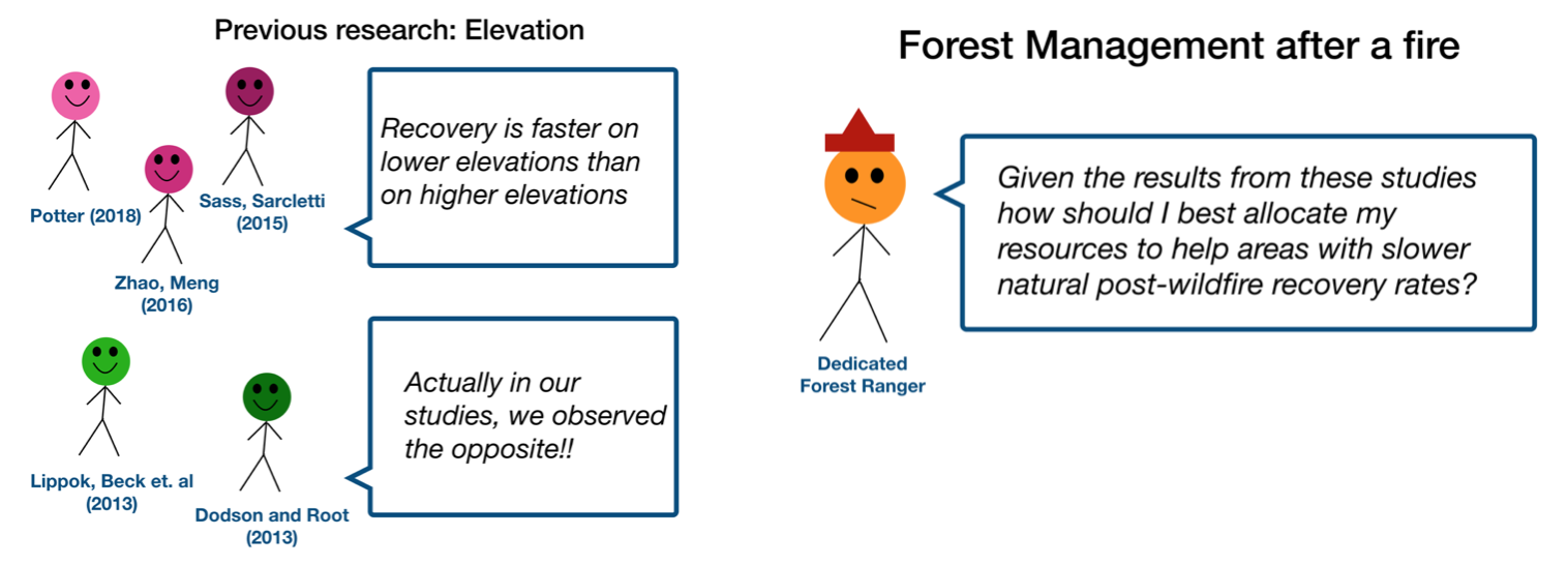
Orient the audience and draw them in by demonstrating the relevance and importance of your research story with strong global motive. Provide them with the necessary vocabulary and background knowledge to understand the plot of your story. Introduce the key studies (characters) relevant in your story and build tension and conflict with scholarly and data motive. By the end of your introduction, your audience should clearly understand your research question and be dying to know how you resolve the tension built through motive.

• Methods (rising action)

The methods section should transition smoothly and logically from the introduction. Beware of presenting your methods in a boring, arc-killing, ‘this is what I did.’ Focus on the details that set your story apart from the stories other people have already told. Keep the audience interested by clearly motivating your decisions based on your original research question or the tension built in your introduction.

• Results (climax)

Less is usually more here. Only present results which are clearly related to the focused research question you are presenting. Make sure you explain the results clearly so that your audience understands what your research found. This is the peak of tension in your narrative arc, so don’t undercut it by quickly clicking through to your discussion.

• Discussion (falling action)

By now your audience should be dying for a satisfying resolution. Here is where you contextualize your results and begin resolving the tension between past research. Be thorough. If you have too many conflicts left unresolved, or you don’t have enough time to present all of the resolutions, you probably need to further narrow the scope of your presentation.

• Conclusion (denouement)

Return back to your initial research question and motive, resolving any final conflicts and tying up loose ends. Leave the audience with a clear resolution of your focus research question, and use unresolved tension to set up potential sequels (i.e. further research).

Use your medium to enhance the narrative

Visual presentations should be dominated by clear, intentional graphics. Subtle animation in key moments (usually during the results or discussion) can add drama to the narrative arc and make conflict resolutions more satisfying. You are narrating a story written in images, videos, cartoons, and graphs. While your paper is mostly text, with graphics to highlight crucial points, your slides should be the opposite. Adapting to the new medium may require you to create or acquire far more graphics than you included in your paper, but it is necessary to create an engaging presentation.

The most important thing you can do for your presentation is to practice and revise. Bother your friends, your roommates, TAs–anybody who will sit down and listen to your work. Beyond that, think about presentations you have found compelling and try to incorporate some of those elements into your own. Remember you want your work to be comprehensible; you aren’t creating experts in 10 minutes. Above all, try to stay passionate about what you did and why. You put the time in, so show your audience that it’s worth it.

For more insight into research presentations, check out these past PCUR posts written by Emma and Ellie .

— Alec Getraer, Natural Sciences Correspondent

Share this:

• Share on Tumblr

Home Blog Design Understanding Data Presentations (Guide + Examples)

Understanding Data Presentations (Guide + Examples)

In this age of overwhelming information, the skill to effectively convey data has become extremely valuable. Initiating a discussion on data presentation types involves thoughtful consideration of the nature of your data and the message you aim to convey. Different types of visualizations serve distinct purposes. Whether you’re dealing with how to develop a report or simply trying to communicate complex information, how you present data influences how well your audience understands and engages with it. This extensive guide leads you through the different ways of data presentation.

Table of Contents

What is a Data Presentation?

What should a data presentation include, line graphs, treemap chart, scatter plot, how to choose a data presentation type, recommended data presentation templates, common mistakes done in data presentation.

A data presentation is a slide deck that aims to disclose quantitative information to an audience through the use of visual formats and narrative techniques derived from data analysis, making complex data understandable and actionable. This process requires a series of tools, such as charts, graphs, tables, infographics, dashboards, and so on, supported by concise textual explanations to improve understanding and boost retention rate.

Data presentations require us to cull data in a format that allows the presenter to highlight trends, patterns, and insights so that the audience can act upon the shared information. In a few words, the goal of data presentations is to enable viewers to grasp complicated concepts or trends quickly, facilitating informed decision-making or deeper analysis.

Data presentations go beyond the mere usage of graphical elements. Seasoned presenters encompass visuals with the art of data storytelling , so the speech skillfully connects the points through a narrative that resonates with the audience. Depending on the purpose – inspire, persuade, inform, support decision-making processes, etc. – is the data presentation format that is better suited to help us in this journey.

To nail your upcoming data presentation, ensure to count with the following elements:

• Clear Objectives: Understand the intent of your presentation before selecting the graphical layout and metaphors to make content easier to grasp.
• Engaging introduction: Use a powerful hook from the get-go. For instance, you can ask a big question or present a problem that your data will answer. Take a look at our guide on how to start a presentation for tips & insights.
• Structured Narrative: Your data presentation must tell a coherent story. This means a beginning where you present the context, a middle section in which you present the data, and an ending that uses a call-to-action. Check our guide on presentation structure for further information.
• Visual Elements: These are the charts, graphs, and other elements of visual communication we ought to use to present data. This article will cover one by one the different types of data representation methods we can use, and provide further guidance on choosing between them.
• Insights and Analysis: This is not just showcasing a graph and letting people get an idea about it. A proper data presentation includes the interpretation of that data, the reason why it’s included, and why it matters to your research.
• Conclusion & CTA: Ending your presentation with a call to action is necessary. Whether you intend to wow your audience into acquiring your services, inspire them to change the world, or whatever the purpose of your presentation, there must be a stage in which you convey all that you shared and show the path to staying in touch. Plan ahead whether you want to use a thank-you slide, a video presentation, or which method is apt and tailored to the kind of presentation you deliver.
• Q&A Session: After your speech is concluded, allocate 3-5 minutes for the audience to raise any questions about the information you disclosed. This is an extra chance to establish your authority on the topic. Check our guide on questions and answer sessions in presentations here.

Bar charts are a graphical representation of data using rectangular bars to show quantities or frequencies in an established category. They make it easy for readers to spot patterns or trends. Bar charts can be horizontal or vertical, although the vertical format is commonly known as a column chart. They display categorical, discrete, or continuous variables grouped in class intervals [1] . They include an axis and a set of labeled bars horizontally or vertically. These bars represent the frequencies of variable values or the values themselves. Numbers on the y-axis of a vertical bar chart or the x-axis of a horizontal bar chart are called the scale.

Real-Life Application of Bar Charts

Let’s say a sales manager is presenting sales to their audience. Using a bar chart, he follows these steps.

Step 1: Selecting Data

The first step is to identify the specific data you will present to your audience.

The sales manager has highlighted these products for the presentation.

• Product A: Men’s Shoes
• Product B: Women’s Apparel
• Product C: Electronics
• Product D: Home Decor

Step 2: Choosing Orientation

Opt for a vertical layout for simplicity. Vertical bar charts help compare different categories in case there are not too many categories [1] . They can also help show different trends. A vertical bar chart is used where each bar represents one of the four chosen products. After plotting the data, it is seen that the height of each bar directly represents the sales performance of the respective product.

It is visible that the tallest bar (Electronics – Product C) is showing the highest sales. However, the shorter bars (Women’s Apparel – Product B and Home Decor – Product D) need attention. It indicates areas that require further analysis or strategies for improvement.

Step 3: Colorful Insights

Different colors are used to differentiate each product. It is essential to show a color-coded chart where the audience can distinguish between products.

• Men’s Shoes (Product A): Yellow
• Women’s Apparel (Product B): Orange
• Electronics (Product C): Violet
• Home Decor (Product D): Blue

Bar charts are straightforward and easily understandable for presenting data. They are versatile when comparing products or any categorical data [2] . Bar charts adapt seamlessly to retail scenarios. Despite that, bar charts have a few shortcomings. They cannot illustrate data trends over time. Besides, overloading the chart with numerous products can lead to visual clutter, diminishing its effectiveness.

For more information, check our collection of bar chart templates for PowerPoint .

Line graphs help illustrate data trends, progressions, or fluctuations by connecting a series of data points called ‘markers’ with straight line segments. This provides a straightforward representation of how values change [5] . Their versatility makes them invaluable for scenarios requiring a visual understanding of continuous data. In addition, line graphs are also useful for comparing multiple datasets over the same timeline. Using multiple line graphs allows us to compare more than one data set. They simplify complex information so the audience can quickly grasp the ups and downs of values. From tracking stock prices to analyzing experimental results, you can use line graphs to show how data changes over a continuous timeline. They show trends with simplicity and clarity.

Real-life Application of Line Graphs

To understand line graphs thoroughly, we will use a real case. Imagine you’re a financial analyst presenting a tech company’s monthly sales for a licensed product over the past year. Investors want insights into sales behavior by month, how market trends may have influenced sales performance and reception to the new pricing strategy. To present data via a line graph, you will complete these steps.

First, you need to gather the data. In this case, your data will be the sales numbers. For example:

• January: $45,000
• February: $55,000
• March: $45,000
• April: $60,000
• May: $ 70,000
• June: $65,000
• July: $62,000
• August: $68,000
• September: $81,000
• October: $76,000
• November: $87,000
• December: $91,000

After choosing the data, the next step is to select the orientation. Like bar charts, you can use vertical or horizontal line graphs. However, we want to keep this simple, so we will keep the timeline (x-axis) horizontal while the sales numbers (y-axis) vertical.

Step 3: Connecting Trends

After adding the data to your preferred software, you will plot a line graph. In the graph, each month’s sales are represented by data points connected by a line.

Step 4: Adding Clarity with Color

If there are multiple lines, you can also add colors to highlight each one, making it easier to follow.

Line graphs excel at visually presenting trends over time. These presentation aids identify patterns, like upward or downward trends. However, too many data points can clutter the graph, making it harder to interpret. Line graphs work best with continuous data but are not suitable for categories.

For more information, check our collection of line chart templates for PowerPoint and our article about how to make a presentation graph .

A data dashboard is a visual tool for analyzing information. Different graphs, charts, and tables are consolidated in a layout to showcase the information required to achieve one or more objectives. Dashboards help quickly see Key Performance Indicators (KPIs). You don’t make new visuals in the dashboard; instead, you use it to display visuals you’ve already made in worksheets [3] .

Keeping the number of visuals on a dashboard to three or four is recommended. Adding too many can make it hard to see the main points [4]. Dashboards can be used for business analytics to analyze sales, revenue, and marketing metrics at a time. They are also used in the manufacturing industry, as they allow users to grasp the entire production scenario at the moment while tracking the core KPIs for each line.

Real-Life Application of a Dashboard

Consider a project manager presenting a software development project’s progress to a tech company’s leadership team. He follows the following steps.

Step 1: Defining Key Metrics

To effectively communicate the project’s status, identify key metrics such as completion status, budget, and bug resolution rates. Then, choose measurable metrics aligned with project objectives.

Step 2: Choosing Visualization Widgets

After finalizing the data, presentation aids that align with each metric are selected. For this project, the project manager chooses a progress bar for the completion status and uses bar charts for budget allocation. Likewise, he implements line charts for bug resolution rates.

Step 3: Dashboard Layout

Key metrics are prominently placed in the dashboard for easy visibility, and the manager ensures that it appears clean and organized.

Dashboards provide a comprehensive view of key project metrics. Users can interact with data, customize views, and drill down for detailed analysis. However, creating an effective dashboard requires careful planning to avoid clutter. Besides, dashboards rely on the availability and accuracy of underlying data sources.

For more information, check our article on how to design a dashboard presentation , and discover our collection of dashboard PowerPoint templates .

Treemap charts represent hierarchical data structured in a series of nested rectangles [6] . As each branch of the ‘tree’ is given a rectangle, smaller tiles can be seen representing sub-branches, meaning elements on a lower hierarchical level than the parent rectangle. Each one of those rectangular nodes is built by representing an area proportional to the specified data dimension.

Treemaps are useful for visualizing large datasets in compact space. It is easy to identify patterns, such as which categories are dominant. Common applications of the treemap chart are seen in the IT industry, such as resource allocation, disk space management, website analytics, etc. Also, they can be used in multiple industries like healthcare data analysis, market share across different product categories, or even in finance to visualize portfolios.

Real-Life Application of a Treemap Chart

Let’s consider a financial scenario where a financial team wants to represent the budget allocation of a company. There is a hierarchy in the process, so it is helpful to use a treemap chart. In the chart, the top-level rectangle could represent the total budget, and it would be subdivided into smaller rectangles, each denoting a specific department. Further subdivisions within these smaller rectangles might represent individual projects or cost categories.

Step 1: Define Your Data Hierarchy

While presenting data on the budget allocation, start by outlining the hierarchical structure. The sequence will be like the overall budget at the top, followed by departments, projects within each department, and finally, individual cost categories for each project.

• Top-level rectangle: Total Budget
• Second-level rectangles: Departments (Engineering, Marketing, Sales)
• Third-level rectangles: Projects within each department
• Fourth-level rectangles: Cost categories for each project (Personnel, Marketing Expenses, Equipment)

Step 2: Choose a Suitable Tool

It’s time to select a data visualization tool supporting Treemaps. Popular choices include Tableau, Microsoft Power BI, PowerPoint, or even coding with libraries like D3.js. It is vital to ensure that the chosen tool provides customization options for colors, labels, and hierarchical structures.

Here, the team uses PowerPoint for this guide because of its user-friendly interface and robust Treemap capabilities.

Step 3: Make a Treemap Chart with PowerPoint

After opening the PowerPoint presentation, they chose “SmartArt” to form the chart. The SmartArt Graphic window has a “Hierarchy” category on the left.  Here, you will see multiple options. You can choose any layout that resembles a Treemap. The “Table Hierarchy” or “Organization Chart” options can be adapted. The team selects the Table Hierarchy as it looks close to a Treemap.

Step 5: Input Your Data

After that, a new window will open with a basic structure. They add the data one by one by clicking on the text boxes. They start with the top-level rectangle, representing the total budget.  

Step 6: Customize the Treemap

By clicking on each shape, they customize its color, size, and label. At the same time, they can adjust the font size, style, and color of labels by using the options in the “Format” tab in PowerPoint. Using different colors for each level enhances the visual difference.

Treemaps excel at illustrating hierarchical structures. These charts make it easy to understand relationships and dependencies. They efficiently use space, compactly displaying a large amount of data, reducing the need for excessive scrolling or navigation. Additionally, using colors enhances the understanding of data by representing different variables or categories.

In some cases, treemaps might become complex, especially with deep hierarchies.  It becomes challenging for some users to interpret the chart. At the same time, displaying detailed information within each rectangle might be constrained by space. It potentially limits the amount of data that can be shown clearly. Without proper labeling and color coding, there’s a risk of misinterpretation.

A heatmap is a data visualization tool that uses color coding to represent values across a two-dimensional surface. In these, colors replace numbers to indicate the magnitude of each cell. This color-shaded matrix display is valuable for summarizing and understanding data sets with a glance [7] . The intensity of the color corresponds to the value it represents, making it easy to identify patterns, trends, and variations in the data.

As a tool, heatmaps help businesses analyze website interactions, revealing user behavior patterns and preferences to enhance overall user experience. In addition, companies use heatmaps to assess content engagement, identifying popular sections and areas of improvement for more effective communication. They excel at highlighting patterns and trends in large datasets, making it easy to identify areas of interest.

We can implement heatmaps to express multiple data types, such as numerical values, percentages, or even categorical data. Heatmaps help us easily spot areas with lots of activity, making them helpful in figuring out clusters [8] . When making these maps, it is important to pick colors carefully. The colors need to show the differences between groups or levels of something. And it is good to use colors that people with colorblindness can easily see.

Check our detailed guide on how to create a heatmap here. Also discover our collection of heatmap PowerPoint templates .

Pie charts are circular statistical graphics divided into slices to illustrate numerical proportions. Each slice represents a proportionate part of the whole, making it easy to visualize the contribution of each component to the total.

The size of the pie charts is influenced by the value of data points within each pie. The total of all data points in a pie determines its size. The pie with the highest data points appears as the largest, whereas the others are proportionally smaller. However, you can present all pies of the same size if proportional representation is not required [9] . Sometimes, pie charts are difficult to read, or additional information is required. A variation of this tool can be used instead, known as the donut chart , which has the same structure but a blank center, creating a ring shape. Presenters can add extra information, and the ring shape helps to declutter the graph.

Pie charts are used in business to show percentage distribution, compare relative sizes of categories, or present straightforward data sets where visualizing ratios is essential.

Real-Life Application of Pie Charts

Consider a scenario where you want to represent the distribution of the data. Each slice of the pie chart would represent a different category, and the size of each slice would indicate the percentage of the total portion allocated to that category.

Step 1: Define Your Data Structure

Imagine you are presenting the distribution of a project budget among different expense categories.

• Column A: Expense Categories (Personnel, Equipment, Marketing, Miscellaneous)
• Column B: Budget Amounts ($40,000, $30,000, $20,000, $10,000) Column B represents the values of your categories in Column A.

Step 2: Insert a Pie Chart

Using any of the accessible tools, you can create a pie chart. The most convenient tools for forming a pie chart in a presentation are presentation tools such as PowerPoint or Google Slides.  You will notice that the pie chart assigns each expense category a percentage of the total budget by dividing it by the total budget.

For instance:

• Personnel: $40,000 / ($40,000 + $30,000 + $20,000 + $10,000) = 40%
• Equipment: $30,000 / ($40,000 + $30,000 + $20,000 + $10,000) = 30%
• Marketing: $20,000 / ($40,000 + $30,000 + $20,000 + $10,000) = 20%
• Miscellaneous: $10,000 / ($40,000 + $30,000 + $20,000 + $10,000) = 10%

You can make a chart out of this or just pull out the pie chart from the data.

3D pie charts and 3D donut charts are quite popular among the audience. They stand out as visual elements in any presentation slide, so let’s take a look at how our pie chart example would look in 3D pie chart format.

Step 03: Results Interpretation

The pie chart visually illustrates the distribution of the project budget among different expense categories. Personnel constitutes the largest portion at 40%, followed by equipment at 30%, marketing at 20%, and miscellaneous at 10%. This breakdown provides a clear overview of where the project funds are allocated, which helps in informed decision-making and resource management. It is evident that personnel are a significant investment, emphasizing their importance in the overall project budget.

Pie charts provide a straightforward way to represent proportions and percentages. They are easy to understand, even for individuals with limited data analysis experience. These charts work well for small datasets with a limited number of categories.

However, a pie chart can become cluttered and less effective in situations with many categories. Accurate interpretation may be challenging, especially when dealing with slight differences in slice sizes. In addition, these charts are static and do not effectively convey trends over time.

For more information, check our collection of pie chart templates for PowerPoint .

Histograms present the distribution of numerical variables. Unlike a bar chart that records each unique response separately, histograms organize numeric responses into bins and show the frequency of reactions within each bin [10] . The x-axis of a histogram shows the range of values for a numeric variable. At the same time, the y-axis indicates the relative frequencies (percentage of the total counts) for that range of values.

Whenever you want to understand the distribution of your data, check which values are more common, or identify outliers, histograms are your go-to. Think of them as a spotlight on the story your data is telling. A histogram can provide a quick and insightful overview if you’re curious about exam scores, sales figures, or any numerical data distribution.

Real-Life Application of a Histogram

In the histogram data analysis presentation example, imagine an instructor analyzing a class’s grades to identify the most common score range. A histogram could effectively display the distribution. It will show whether most students scored in the average range or if there are significant outliers.

Step 1: Gather Data

He begins by gathering the data. The scores of each student in class are gathered to analyze exam scores.

After arranging the scores in ascending order, bin ranges are set.

Step 2: Define Bins

Bins are like categories that group similar values. Think of them as buckets that organize your data. The presenter decides how wide each bin should be based on the range of the values. For instance, the instructor sets the bin ranges based on score intervals: 60-69, 70-79, 80-89, and 90-100.

Step 3: Count Frequency

Now, he counts how many data points fall into each bin. This step is crucial because it tells you how often specific ranges of values occur. The result is the frequency distribution, showing the occurrences of each group.

Here, the instructor counts the number of students in each category.

• 60-69: 1 student (Kate)
• 70-79: 4 students (David, Emma, Grace, Jack)
• 80-89: 7 students (Alice, Bob, Frank, Isabel, Liam, Mia, Noah)
• 90-100: 3 students (Clara, Henry, Olivia)

Step 4: Create the Histogram

It’s time to turn the data into a visual representation. Draw a bar for each bin on a graph. The width of the bar should correspond to the range of the bin, and the height should correspond to the frequency.  To make your histogram understandable, label the X and Y axes.

In this case, the X-axis should represent the bins (e.g., test score ranges), and the Y-axis represents the frequency.

The histogram of the class grades reveals insightful patterns in the distribution. Most students, with seven students, fall within the 80-89 score range. The histogram provides a clear visualization of the class’s performance. It showcases a concentration of grades in the upper-middle range with few outliers at both ends. This analysis helps in understanding the overall academic standing of the class. It also identifies the areas for potential improvement or recognition.

Thus, histograms provide a clear visual representation of data distribution. They are easy to interpret, even for those without a statistical background. They apply to various types of data, including continuous and discrete variables. One weak point is that histograms do not capture detailed patterns in students’ data, with seven compared to other visualization methods.

A scatter plot is a graphical representation of the relationship between two variables. It consists of individual data points on a two-dimensional plane. This plane plots one variable on the x-axis and the other on the y-axis. Each point represents a unique observation. It visualizes patterns, trends, or correlations between the two variables.

Scatter plots are also effective in revealing the strength and direction of relationships. They identify outliers and assess the overall distribution of data points. The points’ dispersion and clustering reflect the relationship’s nature, whether it is positive, negative, or lacks a discernible pattern. In business, scatter plots assess relationships between variables such as marketing cost and sales revenue. They help present data correlations and decision-making.

Real-Life Application of Scatter Plot

A group of scientists is conducting a study on the relationship between daily hours of screen time and sleep quality. After reviewing the data, they managed to create this table to help them build a scatter plot graph:

In the provided example, the x-axis represents Daily Hours of Screen Time, and the y-axis represents the Sleep Quality Rating.

The scientists observe a negative correlation between the amount of screen time and the quality of sleep. This is consistent with their hypothesis that blue light, especially before bedtime, has a significant impact on sleep quality and metabolic processes.

There are a few things to remember when using a scatter plot. Even when a scatter diagram indicates a relationship, it doesn’t mean one variable affects the other. A third factor can influence both variables. The more the plot resembles a straight line, the stronger the relationship is perceived [11] . If it suggests no ties, the observed pattern might be due to random fluctuations in data. When the scatter diagram depicts no correlation, whether the data might be stratified is worth considering.

Choosing the appropriate data presentation type is crucial when making a presentation . Understanding the nature of your data and the message you intend to convey will guide this selection process. For instance, when showcasing quantitative relationships, scatter plots become instrumental in revealing correlations between variables. If the focus is on emphasizing parts of a whole, pie charts offer a concise display of proportions. Histograms, on the other hand, prove valuable for illustrating distributions and frequency patterns. 

Bar charts provide a clear visual comparison of different categories. Likewise, line charts excel in showcasing trends over time, while tables are ideal for detailed data examination. Starting a presentation on data presentation types involves evaluating the specific information you want to communicate and selecting the format that aligns with your message. This ensures clarity and resonance with your audience from the beginning of your presentation.

1. Fact Sheet Dashboard for Data Presentation

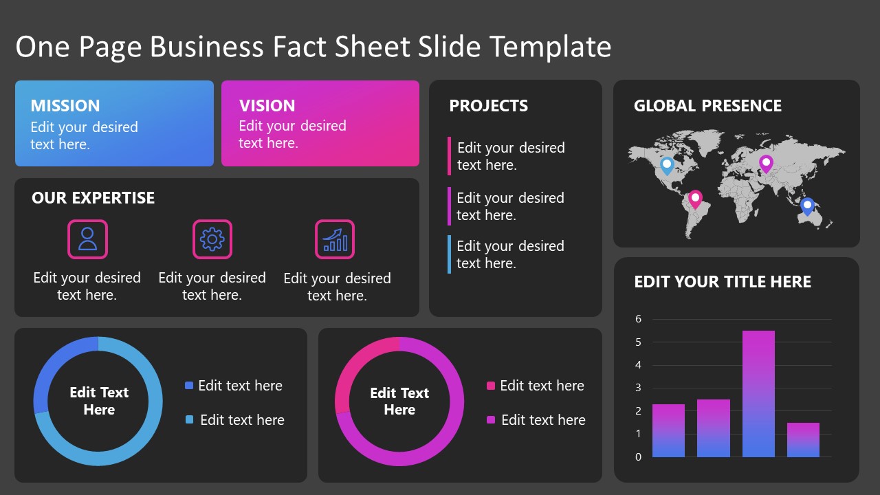
Convey all the data you need to present in this one-pager format, an ideal solution tailored for users looking for presentation aids. Global maps, donut chats, column graphs, and text neatly arranged in a clean layout presented in light and dark themes.

Use This Template

2. 3D Column Chart Infographic PPT Template

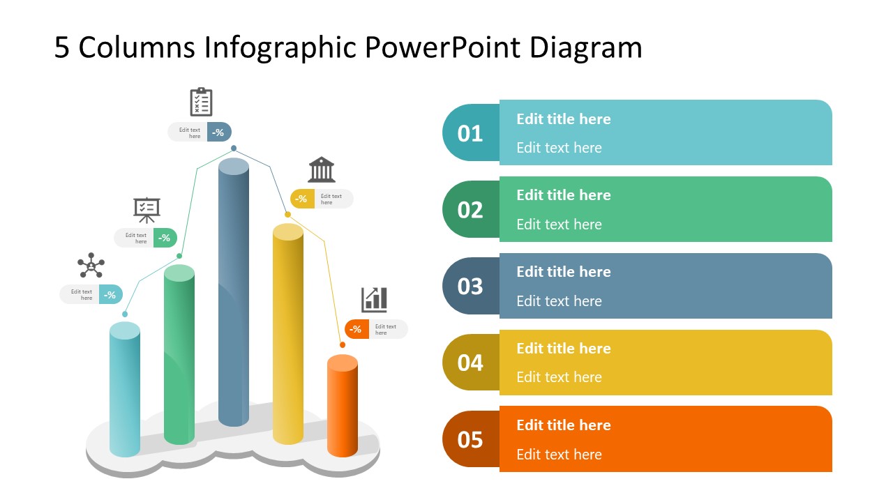
Represent column charts in a highly visual 3D format with this PPT template. A creative way to present data, this template is entirely editable, and we can craft either a one-page infographic or a series of slides explaining what we intend to disclose point by point.

3. Data Circles Infographic PowerPoint Template

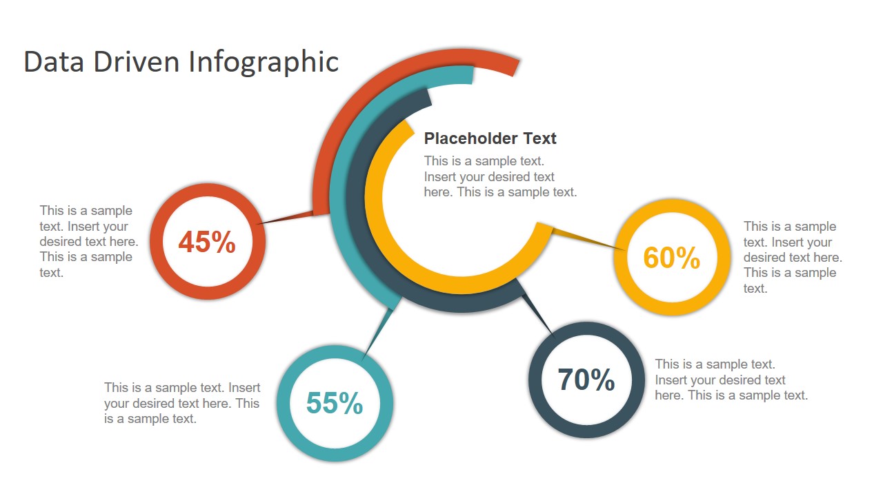
An alternative to the pie chart and donut chart diagrams, this template features a series of curved shapes with bubble callouts as ways of presenting data. Expand the information for each arch in the text placeholder areas.

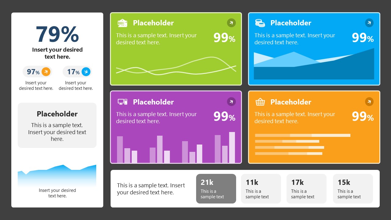
4. Colorful Metrics Dashboard for Data Presentation

This versatile dashboard template helps us in the presentation of the data by offering several graphs and methods to convert numbers into graphics. Implement it for e-commerce projects, financial projections, project development, and more.

5. Animated Data Presentation Tools for PowerPoint & Google Slides

A slide deck filled with most of the tools mentioned in this article, from bar charts, column charts, treemap graphs, pie charts, histogram, etc. Animated effects make each slide look dynamic when sharing data with stakeholders.

6. Statistics Waffle Charts PPT Template for Data Presentations

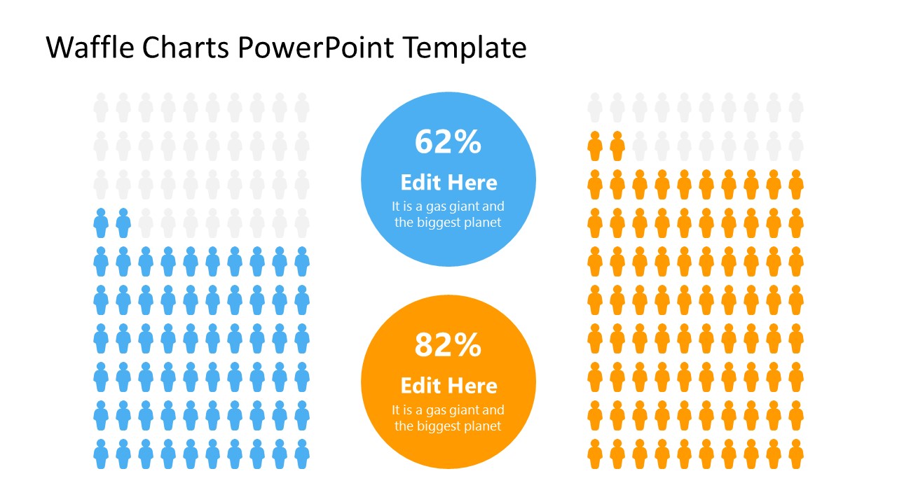
This PPT template helps us how to present data beyond the typical pie chart representation. It is widely used for demographics, so it’s a great fit for marketing teams, data science professionals, HR personnel, and more.

7. Data Presentation Dashboard Template for Google Slides

A compendium of tools in dashboard format featuring line graphs, bar charts, column charts, and neatly arranged placeholder text areas. 

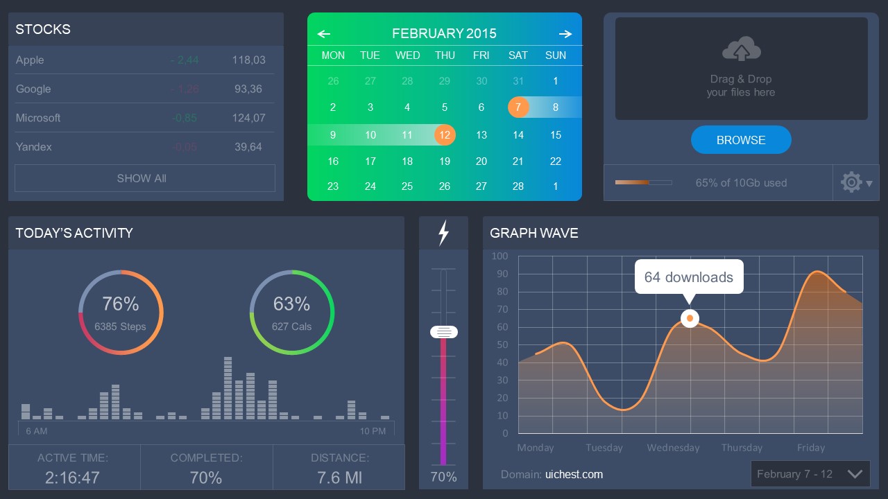
8. Weather Dashboard for Data Presentation

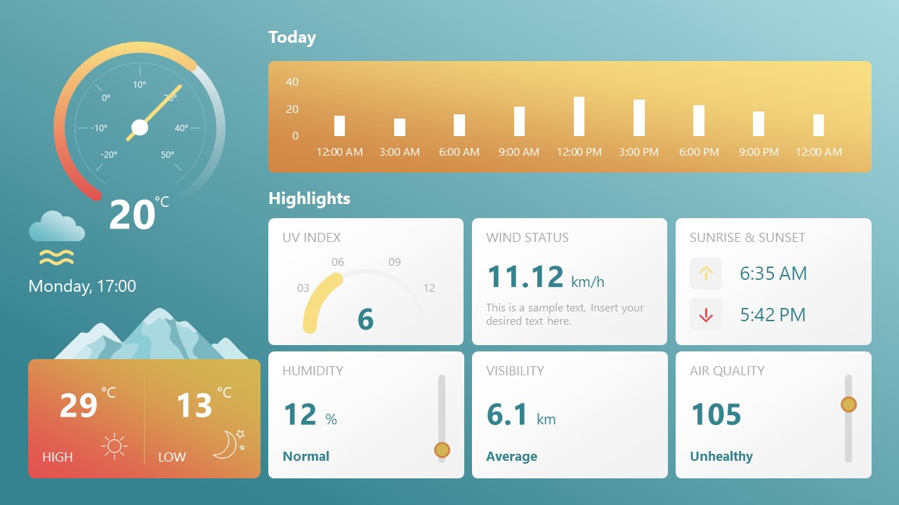
Share weather data for agricultural presentation topics, environmental studies, or any kind of presentation that requires a highly visual layout for weather forecasting on a single day. Two color themes are available.

9. Social Media Marketing Dashboard Data Presentation Template

Intended for marketing professionals, this dashboard template for data presentation is a tool for presenting data analytics from social media channels. Two slide layouts featuring line graphs and column charts.

10. Project Management Summary Dashboard Template

A tool crafted for project managers to deliver highly visual reports on a project’s completion, the profits it delivered for the company, and expenses/time required to execute it. 4 different color layouts are available.

11. Profit & Loss Dashboard for PowerPoint and Google Slides

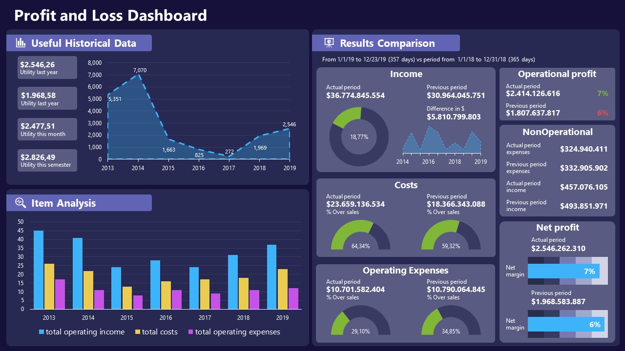
A must-have for finance professionals. This typical profit & loss dashboard includes progress bars, donut charts, column charts, line graphs, and everything that’s required to deliver a comprehensive report about a company’s financial situation.

Overwhelming visuals

One of the mistakes related to using data-presenting methods is including too much data or using overly complex visualizations. They can confuse the audience and dilute the key message.

Inappropriate chart types

Choosing the wrong type of chart for the data at hand can lead to misinterpretation. For example, using a pie chart for data that doesn’t represent parts of a whole is not right.

Lack of context

Failing to provide context or sufficient labeling can make it challenging for the audience to understand the significance of the presented data.

Inconsistency in design

Using inconsistent design elements and color schemes across different visualizations can create confusion and visual disarray.

Failure to provide details

Simply presenting raw data without offering clear insights or takeaways can leave the audience without a meaningful conclusion.

Lack of focus

Not having a clear focus on the key message or main takeaway can result in a presentation that lacks a central theme.

Visual accessibility issues

Overlooking the visual accessibility of charts and graphs can exclude certain audience members who may have difficulty interpreting visual information.

In order to avoid these mistakes in data presentation, presenters can benefit from using presentation templates . These templates provide a structured framework. They ensure consistency, clarity, and an aesthetically pleasing design, enhancing data communication’s overall impact.

Understanding and choosing data presentation types are pivotal in effective communication. Each method serves a unique purpose, so selecting the appropriate one depends on the nature of the data and the message to be conveyed. The diverse array of presentation types offers versatility in visually representing information, from bar charts showing values to pie charts illustrating proportions. 

Using the proper method enhances clarity, engages the audience, and ensures that data sets are not just presented but comprehensively understood. By appreciating the strengths and limitations of different presentation types, communicators can tailor their approach to convey information accurately, developing a deeper connection between data and audience understanding.

[1] Government of Canada, S.C. (2021) 5 Data Visualization 5.2 Bar Chart , 5.2 Bar chart .  https://www150.statcan.gc.ca/n1/edu/power-pouvoir/ch9/bargraph-diagrammeabarres/5214818-eng.htm

[2] Kosslyn, S.M., 1989. Understanding charts and graphs. Applied cognitive psychology, 3(3), pp.185-225. https://apps.dtic.mil/sti/pdfs/ADA183409.pdf

[3] Creating a Dashboard . https://it.tufts.edu/book/export/html/1870

[4] https://www.goldenwestcollege.edu/research/data-and-more/data-dashboards/index.html

[5] https://www.mit.edu/course/21/21.guide/grf-line.htm

[6] Jadeja, M. and Shah, K., 2015, January. Tree-Map: A Visualization Tool for Large Data. In GSB@ SIGIR (pp. 9-13). https://ceur-ws.org/Vol-1393/gsb15proceedings.pdf#page=15

[7] Heat Maps and Quilt Plots. https://www.publichealth.columbia.edu/research/population-health-methods/heat-maps-and-quilt-plots

[8] EIU QGIS WORKSHOP. https://www.eiu.edu/qgisworkshop/heatmaps.php

[9] About Pie Charts.  https://www.mit.edu/~mbarker/formula1/f1help/11-ch-c8.htm

[10] Histograms. https://sites.utexas.edu/sos/guided/descriptive/numericaldd/descriptiven2/histogram/ [11] https://asq.org/quality-resources/scatter-diagram

Like this article? Please share

Data Analysis, Data Science, Data Visualization Filed under Design

Related Articles

Filed under Design • March 27th, 2024

How to Make a Presentation Graph

Detailed step-by-step instructions to master the art of how to make a presentation graph in PowerPoint and Google Slides. Check it out!

Filed under Presentation Ideas • January 6th, 2024

All About Using Harvey Balls

Among the many tools in the arsenal of the modern presenter, Harvey Balls have a special place. In this article we will tell you all about using Harvey Balls.

Filed under Business • December 8th, 2023

How to Design a Dashboard Presentation: A Step-by-Step Guide

Take a step further in your professional presentation skills by learning what a dashboard presentation is and how to properly design one in PowerPoint. A detailed step-by-step guide is here!

Leave a Reply

• Privacy Policy

Home » Graphical Methods – Types, Examples and Guide

Graphical Methods – Types, Examples and Guide

Table of Contents

Graphical Methods

Definition:

Graphical methods refer to techniques used to visually represent data, relationships, or processes using charts, graphs, diagrams, or other graphical formats. These methods are widely used in various fields such as science, engineering, business, and social sciences, among others, to analyze, interpret and communicate complex information in a concise and understandable way.

Types of Graphical Methods

Here are some of the most common types of graphical methods for data analysis and visual presentation:

Line Graphs

These are commonly used to show trends over time, such as the stock prices of a particular company or the temperature over a certain period. They consist of a series of data points connected by a line that shows the trend of the data over time. Line graphs are useful for identifying patterns in data, such as seasonal changes or long-term trends.

These are commonly used to compare values of different categories, such as sales figures for different products or the number of students in different grade levels. Bar charts use bars that are either horizontal or vertical and represent the data values. They are useful for comparing data visually and identifying differences between categories.

These are used to show how a whole is divided into parts, such as the percentage of students in a school who are enrolled in different programs. Pie charts use a circle that is divided into sectors, with each sector representing a portion of the whole. They are useful for showing proportions and identifying which parts of a whole are larger or smaller.

Scatter Plots

These are used to visualize the relationship between two variables, such as the correlation between a person’s height and weight. Scatter plots consist of a series of data points that are plotted on a graph and connected by a line or curve. They are useful for identifying trends and relationships between variables.

These are used to show the distribution of data across a two-dimensional plane, such as a map of a city showing the density of population in different areas. Heat maps use color-coded cells to represent different levels of data, with darker colors indicating higher values. They are useful for identifying areas of high or low density and for highlighting patterns in data.

These are used to show the distribution of data in a single variable, such as the distribution of ages of a group of people. Histograms use bars that represent the frequency of each data value, with taller bars indicating a higher frequency. They are useful for identifying the shape of a distribution and for identifying outliers or unusual data values.

Network Diagrams

These are used to show the relationships between different entities or nodes, such as the relationships between people in a social network. Network diagrams consist of nodes that are connected by lines that represent the relationship. They are useful for identifying patterns in complex data and for understanding the structure of a network.

Box plots, also known as box-and-whisker plots, are a type of graphical method used to show the distribution of data in a single variable. They consist of a box with whiskers extending from the top and bottom of the box. The box represents the middle 50% of the data, with the median value indicated by a line inside the box. The whiskers represent the range of the data, with any data points outside the whiskers indicated as outliers. Box plots are useful for identifying the spread and shape of a distribution and for identifying outliers or unusual data values.

Applications of Graphical Methods

Graphical methods have a wide range of applications in various fields, including:

• Business : Graphical methods are commonly used in business to analyze sales data, financial data, and other types of data. They are useful for identifying trends, patterns, and outliers, as well as for presenting data in a clear and concise manner to stakeholders.
• Science and engineering: Graphical methods are used extensively in scientific and engineering fields to analyze data and to present research findings. They are useful for visualizing complex data sets and for identifying relationships between variables.
• Social sciences: Graphical methods are used in social sciences to analyze and present data related to human behavior, such as demographics, survey results, and statistical analyses. They are useful for identifying trends and patterns in large data sets and for communicating findings to a broader audience.
• Education : Graphical methods are used in education to present information to students and to help them understand complex concepts. They are useful for visualizing data and for presenting information in a way that is easy to understand.
• Healthcare : Graphical methods are used in healthcare to analyze patient data, to track disease outbreaks, and to present medical information to patients. They are useful for identifying patterns and trends in patient data and for communicating medical information in a clear and concise manner.
• Sports : Graphical methods are used in sports to analyze and present data related to player performance, team statistics, and game outcomes. They are useful for identifying trends and patterns in player and team data and for communicating this information to coaches, players, and fans.

Examples of Graphical Methods

Here are some examples of real-time applications of graphical methods:

• Stock Market: Line graphs, candlestick charts, and bar charts are widely used in real-time trading systems to display stock prices and trends over time. Traders use these charts to analyze historical data and make informed decisions about buying and selling stocks in real-time.
• Weather Forecasting : Heat maps and radar maps are commonly used in weather forecasting to display current weather conditions and to predict future weather patterns. These maps are useful for tracking the movement of storms, identifying areas of high and low pressure, and predicting the likelihood of severe weather events.
• Social Media Analytics: Scatter plots and network diagrams are commonly used in social media analytics to track the spread of information across social networks. Analysts use these graphs to identify patterns in user behavior, to track the popularity of specific topics or hashtags, and to monitor the influence of key opinion leaders.
• Traffic Analysis: Heat maps and network diagrams are used in traffic analysis to visualize traffic flow patterns and to identify areas of congestion or accidents. These graphs are useful for predicting traffic patterns, optimizing traffic flow, and improving transportation infrastructure.
• Medical Diagnostics: Box plots and histograms are commonly used in medical diagnostics to display the distribution of patient data, such as blood pressure, heart rate, or blood sugar levels. These graphs are useful for identifying patterns in patient data, diagnosing medical conditions, and monitoring the effectiveness of treatments in real-time.
• Cybersecurity: Heat maps and network diagrams are used in cybersecurity to visualize network traffic patterns and to identify potential security threats. These graphs are useful for identifying anomalies in network traffic, detecting and mitigating cyber attacks, and improving network security protocols.

How to use Graphical Methods

Here are some general steps to follow when using graphical methods to analyze and present data:

• Identify the research question: Before creating any graphs, it’s important to identify the research question or hypothesis you want to explore. This will help you select the appropriate type of graph and ensure that the data you collect is relevant to your research question.
• Collect and organize the data: Collect the data you need to answer your research question and organize it in a way that makes it easy to work with. This may involve sorting, filtering, or cleaning the data to ensure that it is accurate and relevant.
• Select the appropriate graph : There are many different types of graphs available, each with its own strengths and weaknesses. Select the appropriate graph based on the type of data you have and the research question you are exploring. For example, a scatterplot may be appropriate for exploring the relationship between two continuous variables, while a bar chart may be appropriate for comparing categorical data.
• Create the graph: Once you have selected the appropriate graph, create it using software or a tool that allows you to customize the graph based on your needs. Be sure to include appropriate labels and titles, and ensure that the graph is clearly legible.
• Analyze the graph: Once you have created the graph, analyze it to identify patterns, trends, and relationships in the data. Look for outliers or other anomalies that may require further investigation.
• Draw conclusions: Based on your analysis of the graph, draw conclusions about the research question you are exploring. Use the graph to support your conclusions and to communicate your findings to others.
• Iterate and refine: Finally, refine your graph or create additional graphs as needed to further explore your research question. Iteratively refining and revising your graphs can help to ensure that you are accurately representing the data and that you are drawing the appropriate conclusions.

When to use Graphical Methods

Graphical methods can be used in a variety of situations to help analyze, interpret, and communicate data. Here are some general guidelines on when to use graphical methods:

• To identify patterns and trends: Graphical methods are useful for identifying patterns and trends in data, which may be difficult to see in raw data tables or spreadsheets. Graphs can reveal trends that may not be immediately apparent in the data, making it easier to draw conclusions and make predictions.
• To compare data: Graphs can be used to compare data from different sources or over different time periods. Graphical comparisons can make it easier to identify differences or similarities in the data, which can be useful for making decisions and taking action.
• To summarize data : Graphs can be used to summarize large amounts of data in a single visual display. This can be particularly useful when presenting data to a broad audience, as it can help to simplify complex data sets and make them more accessible.
• To communicate data: Graphs can be used to communicate data and findings to a variety of audiences, including stakeholders, colleagues, and the general public. Graphs can be particularly useful in situations where data needs to be presented quickly and in a way that is easy to understand.
• To identify outliers: Graphical methods are useful for identifying outliers or anomalies in the data. Outliers can be indicative of errors or unusual events, and may warrant further investigation.

Purpose of Graphical Methods

The purpose of graphical methods is to help people analyze, interpret, and communicate data in a way that is both accurate and understandable. Graphical methods provide visual representations of data that can be easier to interpret than tables of numbers or raw data sets. Graphical methods help to reveal patterns and trends that may not be immediately apparent in the data, making it easier to draw conclusions and make predictions. They can also help to identify outliers or unusual data points that may warrant further investigation.

In addition to helping people analyze and interpret data, graphical methods also serve an important communication function. Graphs can be used to present data to a wide range of audiences, including stakeholders, colleagues, and the general public. Graphs can help to simplify complex data sets, making them more accessible and easier to understand. By presenting data in a clear and concise way, graphical methods can help people make informed decisions and take action based on the data.

Overall, the purpose of graphical methods is to provide a powerful tool for analyzing, interpreting, and communicating data. Graphical methods help people to better understand the data they are working with, to identify patterns and trends, and to make informed decisions based on the data.

Characteristics of Graphical Methods

Here are some characteristics of graphical methods:

• Visual Representation: Graphical methods provide a visual representation of data, which can be easier to interpret than tables of numbers or raw data sets. Graphs can help to reveal patterns and trends that may not be immediately apparent in the data.
• Simplicity : Graphical methods simplify complex data sets, making them more accessible and easier to understand. By presenting data in a clear and concise way, graphical methods can help people make informed decisions and take action based on the data.
• Comparability : Graphical methods can be used to compare data from different sources or over different time periods. This can help to identify differences or similarities in the data, which can be useful for making decisions and taking action.
• Flexibility : Graphical methods can be adapted to different types of data, including continuous, categorical, and ordinal data. Different types of graphs can be used to display different types of data, depending on the characteristics of the data and the research question.
• Accuracy : Graphical methods should accurately represent the data being analyzed. Graphs should be properly scaled and labeled to avoid distorting the data or misleading viewers.
• Clarity : Graphical methods should be clear and easy to read. Graphs should be designed with the viewer in mind, using appropriate colors, labels, and titles to ensure that the message of the graph is conveyed effectively.

Advantages of Graphical Methods

Graphical methods offer several advantages for analyzing and presenting data, including:

• Clear visualization: Graphical methods provide a clear and intuitive visual representation of data that can help people understand complex relationships, trends, and patterns in the data. This can be particularly useful when dealing with large and complex data sets.
• Efficient communication: Graphical methods can help to communicate complex data sets in an efficient and accessible way. Visual representations can be easier to understand than numerical data alone, and can help to convey key messages quickly.
• Effective comparison: Graphical methods allow for easy comparison between different data sets, making it easier to identify trends, patterns, and differences. This can help in making decisions, identifying areas for improvement, or developing new insights.
• Improved decision-making: Graphical methods can help to inform decision-making by presenting data in a clear and easy-to-understand format. They can also help to identify key areas of focus, enabling individuals or teams to make more informed decisions.
• Increased engagement: Graphical methods can help to engage audiences by presenting data in an engaging and interactive way. This can be particularly useful in presentations or reports, where visual representations can help to maintain audience attention and interest.
• Better understanding: Graphical methods can help individuals to better understand the data they are working with, by providing a clear and intuitive visual representation of the data. This can lead to improved insights and decision-making, as well as better understanding of the implications of the data.

Limitations of Graphical Methods

Here are a few limitations to consider:

• Misleading representation: Graphical methods can potentially misrepresent data if they are not designed properly. For example, inappropriate scaling or labeling of the axes or the use of certain types of graphs can create a distorted view of the data.
• Limited scope: Graphical methods can only display a limited amount of data, which can make it difficult to capture the full complexity of a data set. Additionally, some types of data may be difficult to represent visually.
• Time-consuming : Creating graphs can be a time-consuming process, particularly if multiple graphs need to be created and analyzed. This can be a limitation in situations where time is limited or resources are scarce.
• Technical skills: Some graphical methods require technical skills to create and interpret. For example, certain types of graphs may require knowledge of specialized software or programming languages.
• Interpretation : Interpreting graphs can be subjective, and the same graph can be interpreted in different ways by different people. This can lead to confusion or disagreements when using graphs to communicate data.
• Accessibility : Some graphical methods may not be accessible to all audiences, particularly those with visual impairments. Additionally, some types of graphs may not be accessible to those with limited literacy or numeracy skills.

About the author

Muhammad Hassan

Researcher, Academic Writer, Web developer

You may also like

Cluster Analysis – Types, Methods and Examples

Discriminant Analysis – Methods, Types and...

MANOVA (Multivariate Analysis of Variance) –...

Documentary Analysis – Methods, Applications and...

ANOVA (Analysis of variance) – Formulas, Types...

Substantive Framework – Types, Methods and...

How to Use Creative Data Visualization Techniques for Easy Comprehension of Qualitative Research

“A picture is worth a thousand words!”—an adage used so often stands true even whilst reporting your research data. Research studies with overwhelming data can perhaps be difficult to comprehend by some readers or can even be time-consuming. While presenting quantitative research data becomes easier with the help of graphs, pie charts, etc. researchers face an undeniable challenge whilst presenting qualitative research data. In this article, we will elaborate on effectively presenting qualitative research using data visualization techniques .

Table of Contents

What is Data Visualization?

Data visualization is the process of converting textual information into graphical and illustrative representations. It is imperative to think beyond numbers to get a holistic and comprehensive understanding of research data. Hence, this technique is adopted to help presenters communicate relevant research data in a way that’s easy for the viewer to interpret and draw conclusions.

What Is the Importance of Data Visualization in Qualitative Research?

According to the form in which the data is collected and expressed, it is broadly divided into qualitative data and quantitative data. Quantitative data expresses the size or quantity of data in a countable integer. Unlike quantitative data, qualitative data cannot be expressed in continuous integer values; it refers to data values ​​described in the non-numeric form related to subjects, places, things, events, activities, or concepts.

What Are the Advantages of Good Data Visualization Techniques?

Excellent data visualization techniques have several benefits:

• Human eyes are often drawn to patterns and colors. Moreover, in this age of Big Data , visualization can be considered an asset to quickly and easily comprehend large amounts of data generated in a research study.
• Enables viewers to recognize emerging trends and accelerate their response time on the basis of what is seen and assimilated.
• Illustrations make it easier to identify correlated parameters.
• Allows the presenter to narrate a story whilst helping the viewer understand the data and draw conclusions from it.
• As humans can process visual images better than texts, data visualization techniques enable viewers to remember them for a longer time.

Different Types of Data Visualization Techniques in Qualitative Research

Here are several data visualization techniques for presenting qualitative data for better comprehension of research data.

1. Word Clouds

• Word Clouds is a type of data visualization technique which helps in visualizing one-word descriptions.
• It is a single image composing multiple words associated with a particular text or subject.
• The size of each word indicates its importance or frequency in the data.
• Wordle and Tagxedo are two majorly used tools to create word clouds.

2. Graphic Timelines

• Graphic timelines are created to present regular text-based timelines with pictorial illustrations or diagrams, photos, and other images.
• It visually displays a series of events in chronological order on a timescale.
• Furthermore, showcasing timelines in a graphical manner makes it easier to understand critical milestones in a study.

3. Icons Beside Descriptions

• Rather than writing long descriptive paragraphs, including resembling icons beside brief and concise points enable quick and easy comprehension.

4. Heat Map

• Using a heat map as a data visualization technique better displays differences in data with color variations.
• The intensity and frequency of data is well addressed with the help of these color codes.
• However, a clear legend must be mentioned alongside the heat map to correctly interpret a heat map.
• Additionally, it also helps identify trends in data.

5. Mind Map

• A mind map helps explain concepts and ideas linked to a central idea.
• Allows visual structuring of ideas without overwhelming the viewer with large amounts of text.
• These can be used to present graphical abstracts

Do’s and Don’ts of Data Visualization Techniques

It perhaps is not easy to visualize qualitative data and make it recognizable and comprehensible to viewers at a glance. However, well-visualized qualitative data can be very useful in order to clearly convey the key points to readers and listeners in presentations.

Are you struggling with ways to display your qualitative data? Which data visualization techniques have you used before? Let us know about your experience in the comments section below!

nicely explained

None. And I want to use it from now.

Would it be ideal or suggested to use these techniques to display qualitative data in a thesis perhaps?

Using data visualization techniques in a qualitative research thesis can help convey your findings in a more engaging and comprehensible manner. Here’s a brief overview of how to incorporate data visualization in such a thesis:

Select Relevant Visualizations: Identify the types of data you have (e.g., textual, audio, visual) and the appropriate visualization techniques that can represent your qualitative data effectively. Common options include word clouds, charts, graphs, timelines, and thematic maps.

Data Preparation: Ensure your qualitative data is well-organized and coded appropriately. This might involve using qualitative analysis software like NVivo or Atlas.ti to tag and categorize data.

Create Visualizations: Generate visualizations that illustrate key themes, patterns, or trends within your qualitative data. For example: Word clouds can highlight frequently occurring terms or concepts. Bar charts or histograms can show the distribution of specific themes or categories. Timeline visualizations can help display chronological trends. Concept maps can illustrate the relationships between different concepts or ideas.

Integrate Visualizations into Your Thesis: Incorporate these visualizations within your thesis to complement your narrative. Place them strategically to support your arguments or findings. Include clear and concise captions and labels for each visualization, providing context and explaining their significance.

Interpretation: In the text of your thesis, interpret the visualizations. Explain what patterns or insights they reveal about your qualitative data. Offer meaningful insights and connections between the visuals and your research questions or hypotheses.

Maintain Consistency: Maintain a consistent style and formatting for your visualizations throughout the thesis. This ensures clarity and professionalism.

Ethical Considerations: If your qualitative research involves sensitive or personal data, consider ethical guidelines and privacy concerns when presenting visualizations. Anonymize or protect sensitive information as needed.

Review and Refinement: Before finalizing your thesis, review the visualizations for accuracy and clarity. Seek feedback from peers or advisors to ensure they effectively convey your qualitative findings.

Appendices: If you have a large number of visualizations or detailed data, consider placing some in appendices. This keeps the main body of your thesis uncluttered while providing interested readers with supplementary information.

Cite Sources: If you use specific software or tools to create your visualizations, acknowledge and cite them appropriately in your thesis.

Hope you find this helpful. Happy Learning!

Rate this article Cancel Reply

Your email address will not be published.

Enago Academy's Most Popular Articles

• Reporting Research

Research Interviews: An effective and insightful way of data collection

Research interviews play a pivotal role in collecting data for various academic, scientific, and professional…

Planning Your Data Collection: Designing methods for effective research

Planning your research is very important to obtain desirable results. In research, the relevance of…

• Manuscript Preparation
• Publishing Research

Qualitative Vs. Quantitative Research — A step-wise guide to conduct research

A research study includes the collection and analysis of data. In quantitative research, the data…

Explanatory & Response Variable in Statistics — A quick guide for early career researchers!

Often researchers have a difficult time choosing the parameters and variables (like explanatory and response…

6 Steps to Evaluate the Effectiveness of Statistical Hypothesis Testing

You know what is tragic? Having the potential to complete the research study but not…

Sign-up to read more

Subscribe for free to get unrestricted access to all our resources on research writing and academic publishing including:

• 2000+ blog articles
• 50+ Webinars
• 10+ Expert podcasts
• 50+ Infographics
• 10+ Checklists
• Research Guides

We hate spam too. We promise to protect your privacy and never spam you.

I am looking for Editing/ Proofreading services for my manuscript Tentative date of next journal submission:

As a researcher, what do you consider most when choosing an image manipulation detector?

• SUGGESTED TOPICS
• The Magazine
• Newsletters
• Managing Yourself
• Managing Teams
• Work-life Balance
• The Big Idea
• Data & Visuals
• Reading Lists
• Case Selections
• HBR Learning
• Topic Feeds
• Account Settings
• Email Preferences

Present Your Data Like a Pro

• Joel Schwartzberg

Demystify the numbers. Your audience will thank you.

While a good presentation has data, data alone doesn’t guarantee a good presentation. It’s all about how that data is presented. The quickest way to confuse your audience is by sharing too many details at once. The only data points you should share are those that significantly support your point — and ideally, one point per chart. To avoid the debacle of sheepishly translating hard-to-see numbers and labels, rehearse your presentation with colleagues sitting as far away as the actual audience would. While you’ve been working with the same chart for weeks or months, your audience will be exposed to it for mere seconds. Give them the best chance of comprehending your data by using simple, clear, and complete language to identify X and Y axes, pie pieces, bars, and other diagrammatic elements. Try to avoid abbreviations that aren’t obvious, and don’t assume labeled components on one slide will be remembered on subsequent slides. Every valuable chart or pie graph has an “Aha!” zone — a number or range of data that reveals something crucial to your point. Make sure you visually highlight the “Aha!” zone, reinforcing the moment by explaining it to your audience.

With so many ways to spin and distort information these days, a presentation needs to do more than simply share great ideas — it needs to support those ideas with credible data. That’s true whether you’re an executive pitching new business clients, a vendor selling her services, or a CEO making a case for change.

• JS Joel Schwartzberg oversees executive communications for a major national nonprofit, is a professional presentation coach, and is the author of Get to the Point! Sharpen Your Message and Make Your Words Matter and The Language of Leadership: How to Engage and Inspire Your Team . You can find him on LinkedIn and X. TheJoelTruth

Partner Center

Loading metrics

Open Access

Ten simple rules for effective presentation slides

* E-mail: [email protected]

Affiliation Biomedical Engineering and the Center for Public Health Genomics, University of Virginia, Charlottesville, Virginia, United States of America

• Kristen M. Naegle

Published: December 2, 2021

• https://doi.org/10.1371/journal.pcbi.1009554
• Reader Comments

Citation: Naegle KM (2021) Ten simple rules for effective presentation slides. PLoS Comput Biol 17(12): e1009554. https://doi.org/10.1371/journal.pcbi.1009554

Copyright: © 2021 Kristen M. Naegle. This is an open access article distributed under the terms of the Creative Commons Attribution License , which permits unrestricted use, distribution, and reproduction in any medium, provided the original author and source are credited.

Funding: The author received no specific funding for this work.

Competing interests: The author has declared no competing interests exist.

Introduction

The “presentation slide” is the building block of all academic presentations, whether they are journal clubs, thesis committee meetings, short conference talks, or hour-long seminars. A slide is a single page projected on a screen, usually built on the premise of a title, body, and figures or tables and includes both what is shown and what is spoken about that slide. Multiple slides are strung together to tell the larger story of the presentation. While there have been excellent 10 simple rules on giving entire presentations [ 1 , 2 ], there was an absence in the fine details of how to design a slide for optimal effect—such as the design elements that allow slides to convey meaningful information, to keep the audience engaged and informed, and to deliver the information intended and in the time frame allowed. As all research presentations seek to teach, effective slide design borrows from the same principles as effective teaching, including the consideration of cognitive processing your audience is relying on to organize, process, and retain information. This is written for anyone who needs to prepare slides from any length scale and for most purposes of conveying research to broad audiences. The rules are broken into 3 primary areas. Rules 1 to 5 are about optimizing the scope of each slide. Rules 6 to 8 are about principles around designing elements of the slide. Rules 9 to 10 are about preparing for your presentation, with the slides as the central focus of that preparation.

Rule 1: Include only one idea per slide

Each slide should have one central objective to deliver—the main idea or question [ 3 – 5 ]. Often, this means breaking complex ideas down into manageable pieces (see Fig 1 , where “background” information has been split into 2 key concepts). In another example, if you are presenting a complex computational approach in a large flow diagram, introduce it in smaller units, building it up until you finish with the entire diagram. The progressive buildup of complex information means that audiences are prepared to understand the whole picture, once you have dedicated time to each of the parts. You can accomplish the buildup of components in several ways—for example, using presentation software to cover/uncover information. Personally, I choose to create separate slides for each piece of information content I introduce—where the final slide has the entire diagram, and I use cropping or a cover on duplicated slides that come before to hide what I’m not yet ready to include. I use this method in order to ensure that each slide in my deck truly presents one specific idea (the new content) and the amount of the new information on that slide can be described in 1 minute (Rule 2), but it comes with the trade-off—a change to the format of one of the slides in the series often means changes to all slides.

• PPT PowerPoint slide
• PNG larger image
• TIFF original image

Top left: A background slide that describes the background material on a project from my lab. The slide was created using a PowerPoint Design Template, which had to be modified to increase default text sizes for this figure (i.e., the default text sizes are even worse than shown here). Bottom row: The 2 new slides that break up the content into 2 explicit ideas about the background, using a central graphic. In the first slide, the graphic is an explicit example of the SH2 domain of PI3-kinase interacting with a phosphorylation site (Y754) on the PDGFR to describe the important details of what an SH2 domain and phosphotyrosine ligand are and how they interact. I use that same graphic in the second slide to generalize all binding events and include redundant text to drive home the central message (a lot of possible interactions might occur in the human proteome, more than we can currently measure). Top right highlights which rules were used to move from the original slide to the new slide. Specific changes as highlighted by Rule 7 include increasing contrast by changing the background color, increasing font size, changing to sans serif fonts, and removing all capital text and underlining (using bold to draw attention). PDGFR, platelet-derived growth factor receptor.

https://doi.org/10.1371/journal.pcbi.1009554.g001

Rule 2: Spend only 1 minute per slide

When you present your slide in the talk, it should take 1 minute or less to discuss. This rule is really helpful for planning purposes—a 20-minute presentation should have somewhere around 20 slides. Also, frequently giving your audience new information to feast on helps keep them engaged. During practice, if you find yourself spending more than a minute on a slide, there’s too much for that one slide—it’s time to break up the content into multiple slides or even remove information that is not wholly central to the story you are trying to tell. Reduce, reduce, reduce, until you get to a single message, clearly described, which takes less than 1 minute to present.

Rule 3: Make use of your heading

When each slide conveys only one message, use the heading of that slide to write exactly the message you are trying to deliver. Instead of titling the slide “Results,” try “CTNND1 is central to metastasis” or “False-positive rates are highly sample specific.” Use this landmark signpost to ensure that all the content on that slide is related exactly to the heading and only the heading. Think of the slide heading as the introductory or concluding sentence of a paragraph and the slide content the rest of the paragraph that supports the main point of the paragraph. An audience member should be able to follow along with you in the “paragraph” and come to the same conclusion sentence as your header at the end of the slide.

Rule 4: Include only essential points

While you are speaking, audience members’ eyes and minds will be wandering over your slide. If you have a comment, detail, or figure on a slide, have a plan to explicitly identify and talk about it. If you don’t think it’s important enough to spend time on, then don’t have it on your slide. This is especially important when faculty are present. I often tell students that thesis committee members are like cats: If you put a shiny bauble in front of them, they’ll go after it. Be sure to only put the shiny baubles on slides that you want them to focus on. Putting together a thesis meeting for only faculty is really an exercise in herding cats (if you have cats, you know this is no easy feat). Clear and concise slide design will go a long way in helping you corral those easily distracted faculty members.

Rule 5: Give credit, where credit is due

An exception to Rule 4 is to include proper citations or references to work on your slide. When adding citations, names of other researchers, or other types of credit, use a consistent style and method for adding this information to your slides. Your audience will then be able to easily partition this information from the other content. A common mistake people make is to think “I’ll add that reference later,” but I highly recommend you put the proper reference on the slide at the time you make it, before you forget where it came from. Finally, in certain kinds of presentations, credits can make it clear who did the work. For the faculty members heading labs, it is an effective way to connect your audience with the personnel in the lab who did the work, which is a great career booster for that person. For graduate students, it is an effective way to delineate your contribution to the work, especially in meetings where the goal is to establish your credentials for meeting the rigors of a PhD checkpoint.

Rule 6: Use graphics effectively

As a rule, you should almost never have slides that only contain text. Build your slides around good visualizations. It is a visual presentation after all, and as they say, a picture is worth a thousand words. However, on the flip side, don’t muddy the point of the slide by putting too many complex graphics on a single slide. A multipanel figure that you might include in a manuscript should often be broken into 1 panel per slide (see Rule 1 ). One way to ensure that you use the graphics effectively is to make a point to introduce the figure and its elements to the audience verbally, especially for data figures. For example, you might say the following: “This graph here shows the measured false-positive rate for an experiment and each point is a replicate of the experiment, the graph demonstrates …” If you have put too much on one slide to present in 1 minute (see Rule 2 ), then the complexity or number of the visualizations is too much for just one slide.

Rule 7: Design to avoid cognitive overload

The type of slide elements, the number of them, and how you present them all impact the ability for the audience to intake, organize, and remember the content. For example, a frequent mistake in slide design is to include full sentences, but reading and verbal processing use the same cognitive channels—therefore, an audience member can either read the slide, listen to you, or do some part of both (each poorly), as a result of cognitive overload [ 4 ]. The visual channel is separate, allowing images/videos to be processed with auditory information without cognitive overload [ 6 ] (Rule 6). As presentations are an exercise in listening, and not reading, do what you can to optimize the ability of the audience to listen. Use words sparingly as “guide posts” to you and the audience about major points of the slide. In fact, you can add short text fragments, redundant with the verbal component of the presentation, which has been shown to improve retention [ 7 ] (see Fig 1 for an example of redundant text that avoids cognitive overload). Be careful in the selection of a slide template to minimize accidentally adding elements that the audience must process, but are unimportant. David JP Phillips argues (and effectively demonstrates in his TEDx talk [ 5 ]) that the human brain can easily interpret 6 elements and more than that requires a 500% increase in human cognition load—so keep the total number of elements on the slide to 6 or less. Finally, in addition to the use of short text, white space, and the effective use of graphics/images, you can improve ease of cognitive processing further by considering color choices and font type and size. Here are a few suggestions for improving the experience for your audience, highlighting the importance of these elements for some specific groups:

• Use high contrast colors and simple backgrounds with low to no color—for persons with dyslexia or visual impairment.
• Use sans serif fonts and large font sizes (including figure legends), avoid italics, underlining (use bold font instead for emphasis), and all capital letters—for persons with dyslexia or visual impairment [ 8 ].
• Use color combinations and palettes that can be understood by those with different forms of color blindness [ 9 ]. There are excellent tools available to identify colors to use and ways to simulate your presentation or figures as they might be seen by a person with color blindness (easily found by a web search).
• In this increasing world of virtual presentation tools, consider practicing your talk with a closed captioning system capture your words. Use this to identify how to improve your speaking pace, volume, and annunciation to improve understanding by all members of your audience, but especially those with a hearing impairment.

Rule 8: Design the slide so that a distracted person gets the main takeaway

It is very difficult to stay focused on a presentation, especially if it is long or if it is part of a longer series of talks at a conference. Audience members may get distracted by an important email, or they may start dreaming of lunch. So, it’s important to look at your slide and ask “If they heard nothing I said, will they understand the key concept of this slide?” The other rules are set up to help with this, including clarity of the single point of the slide (Rule 1), titling it with a major conclusion (Rule 3), and the use of figures (Rule 6) and short text redundant to your verbal description (Rule 7). However, with each slide, step back and ask whether its main conclusion is conveyed, even if someone didn’t hear your accompanying dialog. Importantly, ask if the information on the slide is at the right level of abstraction. For example, do you have too many details about the experiment, which hides the conclusion of the experiment (i.e., breaking Rule 1)? If you are worried about not having enough details, keep a slide at the end of your slide deck (after your conclusions and acknowledgments) with the more detailed information that you can refer to during a question and answer period.

Rule 9: Iteratively improve slide design through practice

Well-designed slides that follow the first 8 rules are intended to help you deliver the message you intend and in the amount of time you intend to deliver it in. The best way to ensure that you nailed slide design for your presentation is to practice, typically a lot. The most important aspects of practicing a new presentation, with an eye toward slide design, are the following 2 key points: (1) practice to ensure that you hit, each time through, the most important points (for example, the text guide posts you left yourself and the title of the slide); and (2) practice to ensure that as you conclude the end of one slide, it leads directly to the next slide. Slide transitions, what you say as you end one slide and begin the next, are important to keeping the flow of the “story.” Practice is when I discover that the order of my presentation is poor or that I left myself too few guideposts to remember what was coming next. Additionally, during practice, the most frequent things I have to improve relate to Rule 2 (the slide takes too long to present, usually because I broke Rule 1, and I’m delivering too much information for one slide), Rule 4 (I have a nonessential detail on the slide), and Rule 5 (I forgot to give a key reference). The very best type of practice is in front of an audience (for example, your lab or peers), where, with fresh perspectives, they can help you identify places for improving slide content, design, and connections across the entirety of your talk.

Rule 10: Design to mitigate the impact of technical disasters

The real presentation almost never goes as we planned in our heads or during our practice. Maybe the speaker before you went over time and now you need to adjust. Maybe the computer the organizer is having you use won’t show your video. Maybe your internet is poor on the day you are giving a virtual presentation at a conference. Technical problems are routinely part of the practice of sharing your work through presentations. Hence, you can design your slides to limit the impact certain kinds of technical disasters create and also prepare alternate approaches. Here are just a few examples of the preparation you can do that will take you a long way toward avoiding a complete fiasco:

• Save your presentation as a PDF—if the version of Keynote or PowerPoint on a host computer cause issues, you still have a functional copy that has a higher guarantee of compatibility.
• In using videos, create a backup slide with screen shots of key results. For example, if I have a video of cell migration, I’ll be sure to have a copy of the start and end of the video, in case the video doesn’t play. Even if the video worked, you can pause on this backup slide and take the time to highlight the key results in words if someone could not see or understand the video.
• Avoid animations, such as figures or text that flash/fly-in/etc. Surveys suggest that no one likes movement in presentations [ 3 , 4 ]. There is likely a cognitive underpinning to the almost universal distaste of pointless animations that relates to the idea proposed by Kosslyn and colleagues that animations are salient perceptual units that captures direct attention [ 4 ]. Although perceptual salience can be used to draw attention to and improve retention of specific points, if you use this approach for unnecessary/unimportant things (like animation of your bullet point text, fly-ins of figures, etc.), then you will distract your audience from the important content. Finally, animations cause additional processing burdens for people with visual impairments [ 10 ] and create opportunities for technical disasters if the software on the host system is not compatible with your planned animation.

Conclusions

These rules are just a start in creating more engaging presentations that increase audience retention of your material. However, there are wonderful resources on continuing on the journey of becoming an amazing public speaker, which includes understanding the psychology and neuroscience behind human perception and learning. For example, as highlighted in Rule 7, David JP Phillips has a wonderful TEDx talk on the subject [ 5 ], and “PowerPoint presentation flaws and failures: A psychological analysis,” by Kosslyn and colleagues is deeply detailed about a number of aspects of human cognition and presentation style [ 4 ]. There are many books on the topic, including the popular “Presentation Zen” by Garr Reynolds [ 11 ]. Finally, although briefly touched on here, the visualization of data is an entire topic of its own that is worth perfecting for both written and oral presentations of work, with fantastic resources like Edward Tufte’s “The Visual Display of Quantitative Information” [ 12 ] or the article “Visualization of Biomedical Data” by O’Donoghue and colleagues [ 13 ].

Acknowledgments

I would like to thank the countless presenters, colleagues, students, and mentors from which I have learned a great deal from on effective presentations. Also, a thank you to the wonderful resources published by organizations on how to increase inclusivity. A special thanks to Dr. Jason Papin and Dr. Michael Guertin on early feedback of this editorial.

• View Article
• PubMed/NCBI
• Google Scholar
• 3. Teaching VUC for Making Better PowerPoint Presentations. n.d. Available from: https://cft.vanderbilt.edu/guides-sub-pages/making-better-powerpoint-presentations/#baddeley .
• 8. Creating a dyslexia friendly workplace. Dyslexia friendly style guide. nd. Available from: https://www.bdadyslexia.org.uk/advice/employers/creating-a-dyslexia-friendly-workplace/dyslexia-friendly-style-guide .
• 9. Cravit R. How to Use Color Blind Friendly Palettes to Make Your Charts Accessible. 2019. Available from: https://venngage.com/blog/color-blind-friendly-palette/ .
• 10. Making your conference presentation more accessible to blind and partially sighted people. n.d. Available from: https://vocaleyes.co.uk/services/resources/guidelines-for-making-your-conference-presentation-more-accessible-to-blind-and-partially-sighted-people/ .
• 11. Reynolds G. Presentation Zen: Simple Ideas on Presentation Design and Delivery. 2nd ed. New Riders Pub; 2011.
• 12. Tufte ER. The Visual Display of Quantitative Information. 2nd ed. Graphics Press; 2001.

Graphical Representation

• Reference work entry
• Cite this reference work entry

680 Accesses

Graphical representations encompass a wide variety of techniques that are used to clarify, interpret and analyze data by plotting points and drawing line segments, surfaces and other geometric forms or symbols.

The purpose of a graph is a rapid visualization of a data set. For instance, it should clearly illustrate the general behavior of the phenomenon investigated and highlight any important factors. It can be used, for example, as a means to translate or to complete a  frequency table .

Therefore, graphical representation is a form of data representation.

The concept of plotting a point in coordinate space dates back to at least the ancient Greeks, but we had to wait until the work of Descartes, René for mathematicians to investigate this concept.

According to Royston, E. (1970), a German mathematician named Crome, A.W. was among the first to use graphical representation in statistics . He initially used it as a teaching tool.

In his works Geographisch-statistische Darstellung...

This is a preview of subscription content, log in via an institution to check access.

Access this chapter

• Available as PDF
• Read on any device
• Instant download
• Own it forever

Tax calculation will be finalised at checkout

Purchases are for personal use only

Institutional subscriptions

Crome, A.F.W.: Ueber die Grösse und Bevölkerung der sämtlichen Europäischen Staaten. Weygand, Leipzig (1785)

Google Scholar  

Crome, A.F.W.: Geographisch-statistische Darstellung der Staatskräfte. Weygand, Leipzig (1820)

Fienberg, S.E.: Graphical method in statistics. Am. Stat. 33 , 165–178 (1979)

Article   Google Scholar  

Guerry, A.M.: Essai sur la statistique morale de la France. Crochard, Paris (1833)

Playfair, W.: The Commercial and Political Atlas. Playfair, London (1786)

Royston, E.: A note on the history of the graphical presentation of data. In: Pearson, E.S., Kendall, M. (eds.) Studies in the History of Statistics and Probability, vol. I. Griffin, London (1970)

Schmid, C.F.: Handbook of Graphic Presentation. Ronald Press, New York (1954)

Download references

Rights and permissions

Reprints and permissions

Copyright information

© 2008 Springer-Verlag

About this entry

Cite this entry.

(2008). Graphical Representation. In: The Concise Encyclopedia of Statistics. Springer, New York, NY. https://doi.org/10.1007/978-0-387-32833-1_174

Download citation

DOI : https://doi.org/10.1007/978-0-387-32833-1_174

Publisher Name : Springer, New York, NY

Print ISBN : 978-0-387-31742-7

Online ISBN : 978-0-387-32833-1

eBook Packages : Mathematics and Statistics Reference Module Computer Science and Engineering

Share this entry

Anyone you share the following link with will be able to read this content:

Sorry, a shareable link is not currently available for this article.

Provided by the Springer Nature SharedIt content-sharing initiative

• Publish with us

Policies and ethics

• Find a journal
• Track your research

• Correspondence
• Open access
• Published: 11 April 2008

Graphical presentation of diagnostic information

• Penny F Whiting 1 ,
• Jonathan AC Sterne 1 ,
• Marie E Westwood 2 ,
• Lucas M Bachmann 3 ,
• Roger Harbord 1 ,
• Matthias Egger 4 &
• Jonathan J Deeks 5  

BMC Medical Research Methodology volume  8 , Article number:  20 ( 2008 ) Cite this article

21k Accesses

101 Citations

6 Altmetric

Metrics details

Graphical displays of results allow researchers to summarise and communicate the key findings of their study. Diagnostic information should be presented in an easily interpretable way, which conveys both test characteristics (diagnostic accuracy) and the potential for use in clinical practice (predictive value).

We discuss the types of graphical display commonly encountered in primary diagnostic accuracy studies and systematic reviews of such studies, and systematically review the use of graphical displays in recent diagnostic primary studies and systematic reviews.

We identified 57 primary studies and 49 systematic reviews. Fifty-six percent of primary studies and 53% of systematic reviews used graphical displays to present results. Dot-plot or box-and- whisker plots were the most commonly used graph in primary studies and were included in 22 (39%) studies. ROC plots were the most common type of plot included in systematic reviews and were included in 22 (45%) reviews. One primary study and five systematic reviews included a probability-modifying plot.

Graphical displays are currently underused in primary diagnostic accuracy studies and systematic reviews of such studies. Diagnostic accuracy studies need to include multiple types of graphic in order to provide both a detailed overview of the results (diagnostic accuracy) and to communicate information that can be used to inform clinical practice (predictive value). Work is required to improve graphical displays, to better communicate the utility of a test in clinical practice and the implications of test results for individual patients.

Peer Review reports

Readers of a research report evaluating a diagnostic test may wish to assess the test's characteristics (diagnostic accuracy) or evaluate the impact that its use has on diagnostic decisions (predictive value) for individual patients. Graphical displays of results of test accuracy studies allow researchers to summarise and communicate the key findings of their study. We discuss the types of graphical display commonly encountered in primary diagnostic accuracy studies and systematic reviews of such studies, and systematically review the use of graphical displays in recent diagnostic systematic reviews and primary studies. Table 1 defines the various measures of diagnostic accuracy used.

Types of graphical display

Primary studies.

Figure 1 illustrates four types of graphical display commonly used to present data on diagnostic accuracy for primary diagnostic accuracy studies. We used data from a study of the biochemical tumour marker CA-19-9 antigen to diagnose pancreatic cancer to construct these graphs [ 1 ].

Example graphical displays for primary study data . a. Dot plot. b. Box-and-whisker plot. c. ROC Plot. d. Flow diagram.

Dot plots (Figure 1a ) and Box-and-whisker plots (Figure 1b )

Dot plots are used for test results that take many values, and display the distribution of results in patients with and without the target condition. Box and whisker plots summarise these distributions: the central box covers the interquartile range with the median indicated by the line within the box. The whiskers extend either to the minimum and maximum values or to the most extreme values within 1.5 interquartile ranges of the quartiles, in which case more extreme values are plotted individually [ 2 ]. Sometimes an indication of the threshold used to define a positive test result is included, for example by adding a horizontal line or shading at the relevant point. Such plots can be used to clearly summarise a large volume of data, but are only able to display differences in the distribution of test values between patients with and without the target condition; they do not directly display the diagnostic performance of the test.

Although the CA-19-9 antigen test to diagnose pancreatic cancer (used to construct Figure 1 ) is an example of continuous data, it is also possible to construct similar graphs for categorical test results providing that the number of categories is reasonably large. Alternatively, for smaller numbers of categories, similar information can be conveyed using paired bar charts/histograms. Paired histograms show the distribution of test results in patients with the target condition above the x-axis and the distribution in patients without the target condition below the x-axis. These types of graphical display are less commonly used. It is not possible to construct any of these graphs for truly dichotomous test results. However, truly dichotomous tests rarely occur in practice. Examples of dichotomous tests include dipstick tests that change colour if the target condition is said to be present (although these are based on an underlying implicit threshold) or the presence/absence of certain clinical symptoms.

Receiver operating characteristic (ROC) plot (Figure 1c )

ROC plots show values of sensitivity and specificity at all of the possible thresholds that could be used to define a positive test result [ 3 ]. Typically, sensitivity (true positive rate) is plotted against 1-specificity (false positive rate): each point represents a different threshold in the same group of patients. Stepped lines are used for continuous test results while sloping lines are used for ordered categories. ROC curves may be derived directly from the observed sensitivity and specificity corresponding to different test thresholds, or by fitting curves based on parametric [ 4 ], semi-parametric [ 5 , 6 ], or non-parametric methods [ 7 ]. The area under the ROC curve (AUC) is a summary of diagnostic performance, and takes values between 0.5 and 1. The more accurate the test, the more closely the curve approaches the top left hand corner of the graph (AUC = 1). A test that provides no diagnostic information (AUC = 0.5) will produce a straight line from the bottom left to the top right. ROC curves may be restricted to a range of sensitivities or specificities of clinical interest.

ROC plots show how estimated sensitivity and specificity vary according to the threshold chosen, and can be used to identify suitable thresholds for clinical practice if the points on the curve are labelled with the corresponding threshold as in Figure 1c , which shows for example that the sensitivity and specificity corresponding to a threshold of 39.3 are 74% and 90%, respectively. Confidence intervals can be added to indicate the uncertainty in estimates of test performance at each point. ROC plots also allow comparison of the performance of several tests independently of choice of threshold, by plotting data sets for multiple tests in the same ROC space. However, they are thought to be difficult to interpret as they describe the characteristics of the test in a way which does not relate directly to its usefulness in clinical practice; research has shown that ROC plots are generally poorly understood by clinicians [ 8 ].

Flow charts (Figure 1d )

These depict the flow of patients through the study: for example how many patients were eligible, how many entered the study, how many of these had the target condition, and the numbers testing positive and negative. Such charts require categorisation of test results, for example as "positive" and "negative". Although flow charts do not directly present diagnostic accuracy data, addition of percentages to the test result boxes (as in Figure 1d ) can be used to report test sensitivity (68/90 = 76%) and specificity (46/51 = 90%). Charts that first separate individuals according to test result before classification by disease status may similarly be used to depict positive and negative predictive values. The STARD (standards for reporting of diagnostic accuracy) statement, an initiative to improve the reporting of diagnostic test accuracy studies similar to the CONSORT statement for clinical trials, recommends the inclusion of a flow diagram in all reports of primary diagnostic accuracy studies [ 9 ]. This should illustrate the design of the study and provide information on the numbers of participants at each stage of the study as well as the results of the study. The example flow chart in Figure 1d is not a full STARD flow diagram as we do not have data on numbers of withdrawals or uninterpretable results from this study. It does, however, show the design (diagnostic case-control) and results of the study.

Systematic reviews

Figure 2 illustrates two graphical displays commonly used to present data on diagnostic accuracy in diagnostic systematic reviews. Data from a systematic review of dipstick tests for urinary nitrite and leukocyte esterase to diagnose urinary tract infections were used to construct these graphs [ 10 ].

Example graphs for systematic review data . a. Paired forest plots of sensitivity and specificity for LE dipstick. b. ROC plot with SROC curves.

Forest plots (Figure 2a )

Forest plots are commonly used to display results of meta-analysis. They display results from the individual studies together with, optionally, a summary (pooled) estimate. Point estimates are shown as dots or squares (sometimes sized according to precision or sample size) and confidence intervals as horizontal lines [ 11 ]. The pooled estimate is displayed as a diamond whose centre represents the estimate and tips the confidence interval.

For diagnostic accuracy studies, measures of test performance (sensitivity, specificity, predictive values, likelihood ratios or diagnostic odds ratio) are plotted on the horizontal axis. Diagnostic test performance is often described by pairs of summary statistics (e.g. sensitivity and specificity; positive and negative likelihood ratios), and these are depicted side-by-side. Between-study heterogeneity can readily be assessed by visual examination. Results may be sorted by one of a pair of test performance measures, usually that which is most important to the clinical application of the test. A disadvantage of paired forest plots is that they do not directly display the inverse association between the two measures that commonly results from variations in threshold between studies.

ROC plots and summary ROC (SROC) curves (Figure 2b )

ROC plots can be used to present the results of diagnostic systematic reviews, but differ from those used in primary studies as each point typically represents a separate study or data set within a study (individual studies may contribute more than one point). A summary ROC (SROC) curve can be estimated using one of several methods [ 12 – 15 ] and quantifies test accuracy and the association between sensitivity and specificity based on differences between studies. As with forest plots, ROC plots provide an overview of the results of all included studies. However, unless there are very few studies, it is not feasible to display confidence intervals as the plot would become cluttered. Results for several tests can be displayed on the same plot, facilitating test comparisons. It is also possible to display pooled estimates of sensitivity and specificity together with associated confidence intervals or prediction regions. ROC plots may also be used to investigate possible explanations for differences in estimates of accuracy between studies, for example those arising from differences in study quality. Figure 3 shows results for a recent review that we conducted on the accuracy of magnetic resonance imaging (MRI) for the diagnosis of multiple sclerosis (MS) [ 16 ]. By using different symbols to illustrate studies that did (diagnostic cohort studies) and did not (other study designs) include an appropriate patient spectrum we were able to show that studies that included an inappropriate patient spectrum grossly overestimated both sensitivity and specificity.

Sensitivity plotted against specificity, separately for cohort studies and for studies of other designs for MRI for diagnosis of multiple sclerosis.

Other plots

Various other graphical methods have been developed to display the results of systematic reviews and meta-analyses [ 17 , 18 ]. Although not generally developed specifically for diagnostic test reviews these can be adapted to display the results of such reviews. Funnel plots [ 19 ] and Galbraith plots [ 20 ] are often used to assess evidence for publication bias or small study effects in systematic reviews of the effects of medical interventions assessed in randomized controlled trials. However, their application to systematic reviews of diagnostic test accuracy studies is problematic [ 20 ]. Diagnostic odds ratios are typically far from 1, and it has been shown that, for data of this type, sampling variation can lead to artefactual associations between log odds ratios and their standard errors [ 21 ]. It is therefore recommended that the effective sample size funnel plot be used in reviews of test accuracy studies [ 20 ].

Predictive value

A number of graphical displays aim to put results of diagnostic test evaluations into clinical context, based either on primary studies or systematic reviews. Two graphical displays commonly used for this purpose are the likelihood ratio nomogram (Figure 4a ) and the probability-modifying plot (Figure 4b ). Each allows the reader to estimate the post-test probability of the target condition in an individual patient, based on a selected pre-test probability. To use the likelihood ratio nomogram, the reader needs an estimate of the likelihood ratios for the test. He then draws a line through the appropriate likelihood ratio on the central axis, intersecting the selected pre-test probability, to derive the post-test probability of disease. The probability-modifying plot depicts separate curves for positive and negative test results. The reader draws a vertical line from the selected pre-test probability to the appropriate likelihood ratio line and then reads the post-test probability off the vertical scale. Both graph types are based on a single estimate of test accuracy (likelihood ratio), although it is possible to plot separate curves on the probability-modifying plot or lines on the nomogram to depict confidence intervals around the estimated likelihood ratios. Each assumes constant likelihood ratios across the range of pre-test probabilities. However, this assumption may be violated in practice [ 22 ], because populations in which the test is used may have different spectrums of disease to those in which estimates of test accuracy were derived.

Example graphs for interpreting diagnostic study result . a. Likelihood ratio nomogram. b. Probability modifying plot.

Use of graphical displays in the literature

We systematically reviewed how graphical displays are currently incorporated in studies of test performance. We included primary diagnostic accuracy studies published in 2004, identified by hand searching 12 journals (Table 2 ), and diagnostic systematic reviews published in 2003, identified from DARE (Database of Abstracts of Reviews of Effects) [ 23 ]. Searches were conducted in 2005 and so these years were the most complete available years for searching (there is a delay in adding studies to DARE). Diagnostic accuracy studies were studies that provided data on the sensitivity and specificity of a diagnostic test and that focused on diagnostic (whether the patient had the condition of interest) rather than prognostic (disease severity/risk prediction) questions. Journals were selected to provide a mixture of the major general medical and specialty journals. We particularly aimed to select journals that clinicians read. We extracted data on the different graphical displays used to summarise information about test performance, defined as any graphical method of summarising data on diagnostic accuracy or the predictive value of a test (Table 1 ).

We located 56 primary studies and 49 systematic reviews (Web Appendix). Fifty-seven percent of primary studies and 53% of systematic reviews used graphical displays to present results. In publications using graphics, the number of graphs per publication ranged from 1 to 51 (median 2, IQR 1 to 3 for primary studies and median 4, IQR 2 to 7 for systematic reviews). Table 3 summarises the categories of tests evaluated in the primary studies and systematic reviews. None of the tests evaluated in any of the primary studies were truly dichotomous: they all gave continuous or categorical results. Three of the eight systematic reviews that assessed clinical examination looked at whether a variety of signs or symptoms were present or absent: these can be considered as truly dichotomous tests. All other reviews evaluated continuous or categorical tests.

Dot-plots or box-and-whisker plots were the most commonly used graphic and were included in 22 (39%) studies. Generally the plots showed individual test results separately for patients with and without the target condition, with four including an indication of the threshold used to define a positive test result. Three studies included both a dot plot and a box-and-whisker plot on the same figure. Other variations included separate plots for different patient subgroups, different symbols to indicate different stages of disease, or separate plots for different tests. The majority of studies using these types of plots were of laboratory tests. An ROC curve was displayed in 15 (26%) studies. All of these plotted full ROC curves; only two provided any indication of the thresholds corresponding to one or more of the points. Thirteen studies included separate ROC curves for different tests, either on the same plot (10 studies) or on separate plots (3 studies). Five studies included separate ROC plots for different patient subgroups. Although all the primary studies were published in 2004, after the publication of the STARD guidelines, only one included a STARD flow diagram.

ROC plots were included in 22 (45%) reviews. Twenty showed individual study estimates of sensitivity and specificity, 14 fitted SROC curves, and two displayed a summary point. One study, which did not fit an SROC curve, added a box and whisker plot to each axis to show the distributions of sensitivity and specificity. One study plotted only summary estimates of sensitivity and specificity in ROC space, with no SROC curves. Some reviews included separate plots for different tests, for different patient subgroups, or for different thresholds used to define a positive test result.

Ten reviews (20%) used forest plots to display individual study results. One study provided a plot of diagnostic odds ratios, while all others displayed paired plots of sensitivity and specificity (8 reviews), positive and negative likelihood ratios (3 reviews), or positive and negative predictive values (1 review). Several studies displayed more than one set of forest plots, including plots for more than one summary measure, for different stages of diagnosis, different test thresholds or for different tests. One study included a forest plot of summary data only, showing how pooled estimates of positive and negative likelihood ratios varied for different patient subgroups.

None of the studies included a likelihood ratio nomogram. One primary study and five systematic reviews included a probability-modifying plot.

Research in the area of cognitive psychology suggests that sensitivity and specificity are generally poorly understood by doctors [ 8 , 24 ] and are often confused with predictive values [ 8 , 25 , 26 ]. Doctors tend to overestimate the impact of a positive test result on the probability of disease [ 27 , 28 ] and this overestimation increases with decreasing pre-test probabilities of disease [ 29 ]. This research suggests that the most informative measures for doctors may be estimates of the post-test probability of disease (predictive value), which can be presented as a range corresponding to different pre-test probabilities. However, graphical displays that facilitate the derivation of post-test probabilities, such as likelihood ratio nomograms, are usually based on summary estimates of test characteristics (positive and negative likelihood ratios) without allowing for the precision of the estimate, or its applicability to a given population. Use of summary estimates in this way is questionable in the context of reviews of diagnostic accuracy studies, which typically find substantial between-study heterogeneity [ 30 ]. It is particularly problematic if the summary estimate is the only information conveyed in a graphic and the graphic is taken as the key message of the paper.

The inclusion of some form of graphical presentation of test accuracy data has a number of advantages compared to not using such displays. It allows fuller reporting of results, for example (S)ROC plots can display results for multiple thresholds whereas reporting test accuracy results in a text or table generally requires the selection of one or more thresholds. In addition, (S)ROC plots depict the trade-off between sensitivity and specificity at different thresholds. Use of such displays also have the advantage of presenting all of the results of a primary study or systematic review without the need for selected analyses, which may be biased depending on the analyses selected. The inclusion of graphical displays, such as SROC plots or forest plots, in systematic reviews of test accuracy studies allows a visual assessment of heterogeneity between studies by showing the results from each individual study included in the review. There is also a suggestion that graphical displays may be easier to interpret than text or tabular summaries of the same data.

Diagnostic accuracy studies will usually need to include more than one graphic in order both to provide a detailed description of results (diagnostic accuracy) and to communicate appropriate summary measures that can be used to inform clinical practice (predictive value); the more detailed graphic provides context for the interpretation of summary measures. Further work is required to improve on existing graphical displays. The starting point for this should be further evaluation of the types of graphical display most helpful to assessing the utility of a test in clinical practice and the implications of test results for individual patients.

We hope that this paper will contribute to an increase in the use and quality of graphical displays in diagnostic accuracy studies and systematic reviews of these studies. To achieve this, journal guidelines and the STARD statement need to encourage the use of graphs in reports of test accuracy. Currently, journal guidelines say very little about this issue. A brief review of the instructions for authors from a selection of leading medical journals ( Annals of Internal Medicine , BMJ , Clinical Chemistry , JAMA , Lancet , New England Journal of Medicine ) found that these only provide formatting guidelines rather than discussing when and what type of graphical displays should be used, although all except the New England Journal of Medicine recommend that the STARD guidelines be followed and include references to the STARD flow diagram. STARD itself does not comment on how graphical displays should be used to convey results of test accuracy studies other than to recommend the inclusion of a flow diagram and to provide an illustration of a dot-plot as a suggestion for how individual study results may be displayed. Guidelines on the type of graphical displays that should be included in reports of test accuracy studies could be considered when STARD is next updated, and should be considered by journals in their instructions for authors.

Our review suggests that graphical displays are currently underused in primary diagnostic accuracy studies and systematic reviews of such studies. Graphical displays of diagnostic accuracy data should provide an easily interpretable and accurate representation of study results, conveying both diagnostic accuracy and predictive value. This is not usually possible in a single graphic: the type of information presented in the most commonly used graphs does not directly allow clinicians to assess the implications of test results for an individual patient.

Web Appendix: Studies included in the review

A. primary studies.

1. Arvanitakis M, Delhaye M, De Maertelaere V, Bali M, Winant C, Coppens E, et al. Computed tomography and magnetic resonance imaging in the assessment of acute pancreatitis. Gastroenterology 2004;126:715–723.

2. Baldas V, Tommasini A, Santon D, Not T, Gerarduzzi T, Clarich G, et al. Testing for Anti-Human Transglutaminase Antibodies in Saliva Is Not Useful for Diagnosis of Celiac Disease. Clin Chem 2004;50:216–219.

3. Banks E, Reeves G, Beral V, Bull D, Crossley B, Simmonds M, et al. Influence of personal characteristics of individual women on sensitivity and specificity of mammography in the Million Women Study: cohort study. BMJ 2004;329:477.

4. Baschat AA, Guclu S, Kush ML, Gembruch U, Weiner CP, Harman CR. Venous Doppler in the prediction of acid-base status of growth-restricted fetuses with elevated placental blood flow resistance. Am J Obstet Gynecol 2004;191:277–284.

5. Biel SS, Nitsche A, Kurth A, Siegert W, Ozel M, Gelderblom HR. Detection of Human Polyomaviruses in Urine from Bone Marrow Transplant Patients: Comparison of Electron Microscopy with PCR. Clin Chem 2004;50:306–312.

6. Bluemke DA, Gatsonis CA, Chen MH, DeAngelis GA, DeBruhl N, Harms S, et al. Magnetic Resonance Imaging of the Breast Prior to Biopsy. JAMA 2004;292:2735–2742.

7. Brugge WR, Lewandrowski K, Lee-Lewandrowski E, Centeno BA, Szydlo T, Regan S, et al. Diagnosis of pancreatic cystic neoplasms: a report of the cooperative pancreatic cyst study. Gastroenterology 2004;126:1330–1336.

8. Bulterys M, Jamieson DJ, O'Sullivan MJ, Cohen MH, Maupin R, Nesheim S, et al. Rapid HIV-1 Testing During Labor: A Multicenter Study. JAMA 2004;292:219–223.

9. Carnevale V, Dionisi S, Nofroni I, Romagnoli E, Paglia F, De Geronimo S, et al. Potential Clinical Utility of a New IRMA for Parathyroid Hormone in Postmenopausal Patients with Primary Hyperparathyroidism. Clin Chem 2004;50:626–631.

10. Chye SM, Lin SR, Chen YL, Chung LY, Yen CM. Immuno-PCR for Detection of Antigen to Angiostrongylus cantonensis Circulating Fifth-Stage Worms. Clin Chem 2004;50:51–57.

11. Cotton PB, Durkalski VL, Pineau BC, Palesch YY, Mauldin PD, Hoffman B, et al. Computed Tomographic Colonography (Virtual Colonoscopy): A Multicenter Comparison With Standard Colonoscopy for Detection of Colorectal Neoplasia. JAMA 2004;291:1713–1719.

12. DeWitt J, Devereaux B, Chriswell M, McGreevy K, Howard T, Imperiale TF, et al. Comparison of Endoscopic Ultrasonography and Multidetector Computed Tomography for Detecting and Staging Pancreatic Cancer. Ann Intern Med 2004;141:753–763.

13. Esteban A, Fernandez-Segoviano P, Frutos-Vivar F, Aramburu JA, Najera L, Ferguson ND, et al. Comparison of Clinical Criteria for the Acute Respiratory Distress Syndrome with Autopsy Findings. Ann Intern Med 2004;141:440–445.

14. Foxman EF, Jarolim P. Use of the Fetal Fibronectin Test in Decisions to Admit to Hospital for Preterm Labor. Clin Chem 2004;50:663–665.

15. Gibot S, Cravoisy A, Levy B, Bene MC, Faure G, Bollaert PE. Soluble Triggering Receptor Expressed on Myeloid Cells and the Diagnosis of Pneumonia. NEJM 2004;350:451–458.

16. Greenough A, Thomas M, Dimitriou G, Williams O, Johnson A, Limb E, et al. Prediction of outcome from the chest radiograph appearance on day 7 of very prematurely born infants. Eur J Pediatr 2004;163:14–18.

17. Grenache DG, Hankins K, Parvin CA, Gronowski AM. Cervicovaginal Interleukin-6, Tumor Necrosis Factor-, and Interleukin-2 Receptor as Markers of Preterm Delivery. Clin Chem 2004;50:1839–1842.

18. Hammerer-Lercher A, Ludwig W, Falkensammer G, Muller S, Neubauer E, Puschendorf B, et al. Natriuretic Peptides as Markers of Mild Forms of Left Ventricular Dysfunction: Effects of Assays on Diagnostic Performance of Markers. Clin Chem 2004;50:1174–1183.

19. Hattori H, Kujiraoka T, Egashira T, Saito E, Fujioka T, Takahashi S, et al. Association of Coronary Heart Disease with Pre-[beta]-HDL Concentrations in Japanese Men. Clin Chem 2004;50:589–595.

20. Herget-Rosenthal S, Poppen D, Husing J, Marggraf G, Pietruck F, Jakob HG, et al. Prognostic Value of Tubular Proteinuria and Enzymuria in Nonoliguric Acute Tubular Necrosis. Clin Chem 2004;50:552–558.

21. Hetzel M, Hetzel J, Arslandemir C, Nussle K, Schirrmeister H. Reliability of symptoms to determine use of bone scans to identify bone metastases in lung cancer: prospective study. BMJ 2004;328:1051–1052.

22. Hift RJ, Davidson BP, van der Hooft C, Meissner DM, Meissner PN. Plasma Fluorescence Scanning and Fecal Porphyrin Analysis for the Diagnosis of Variegate Porphyria: Precise Determination of Sensitivity and Specificity with Detection of Protoporphyrinogen Oxidase Mutations as a Reference Standard. Clin Chem 2004;50:915–923.

23. Hong KM, Najjar H, Hawley M, Press RD. Quantitative Real-Time PCR with Automated Sample Preparation for Diagnosis and Monitoring of Cytomegalovirus Infection in Bone Marrow Transplant Patients. Clin Chem 2004;50:846–856.

24. Imperiale TF, Ransohoff DF, Itzkowitz SH, Turnbull BA, Ross ME, the Colorectal Cancer Study Group. Fecal DNA versus Fecal Occult Blood for Colorectal-Cancer Screening in an Average-Risk Population. NEJM 2004;351:2704–2714.

25. Jung K, Reiche J, Boehme A, Stephan C, Loening SA, Schnorr D, et al. Analysis of Subforms of Free Prostate-Specific Antigen in Serum by Two-Dimensional Gel Electrophoresis: Potential to Improve Diagnosis of Prostate Cancer. Clin Chem 2004;50:2292–2301.

26. Kageyama S, Isono T, Iwaki H, Wakabayashi Y, Okada Y, Kontani K, et al. Identification by Proteomic Analysis of Calreticulin as a Marker for Bladder Cancer and Evaluation of the Diagnostic Accuracy of Its Detection in Urine. Clin Chem 2004;50:857–866.

27. Kiesslich R, Burg J, Vieth M, Gnaendiger J, Enders M, Delaney P, et al. Confocal laser endoscopy for diagnosing intraepithelial neoplasias and colorectal cancer in vivo. Gastroenterology 2004;127:706–713.

28. Kramer H, van Putten JWG, Post WJ, van Dullemen HM, Bongaerts AHH, Pruim J, et al. Oesophageal endoscopic ultrasound with fine needle aspiration improves and simplifies the staging of lung cancer. Thorax 2004;59:596–601.

29. Kriege M, Brekelmans CTM, Boetes C, Besnard PE, Zonderland HM, Obdeijn IM, et al. Efficacy of MRI and Mammography for Breast-Cancer Screening in Women with a Familial or Genetic Predisposition. NEJM 2004;351:427–437.

30. Lacey JM, Minutti CZ, Magera MJ, Tauscher AL, Casetta B, McCann M, et al. Improved Specificity of Newborn Screening for Congenital Adrenal Hyperplasia by Second-Tier Steroid Profiling Using Tandem Mass Spectrometry. Clin Chem 2004;50:621–625.

31. Lennon PV, Wingerchuk DM, Kryzer TJ, Pittock SJ, Lucchinetti CF, Fujihara K, et al. A serum autoantibody marker of neuromyelitis optica: distinction from multiple sclerosis. Lancet 2004;364:2106–2112.

32. Leung Sf, Tam JS, Chan ATC, Zee B, Chan LYS, Huang DP, et al. Improved Accuracy of Detection of Nasopharyngeal Carcinoma by Combined Application of Circulating Epstein-Barr Virus DNA and Anti-Epstein-Barr Viral Capsid Antigen IgA Antibody. Clin Chem 2004;50:339–345.

33. Leung GM, Rainer TH, Lau FL, Wong IOL, Tong A, Wong TW, et al. A Clinical Prediction Rule for Diagnosing Severe Acute Respiratory Syndrome in the Emergency Department. Ann Intern Med 2004;141:333–342.

35. Liebeschuetz S, Bamber S, Ewer K, Deeks J, Pathan AA, Lalvani A. Diagnosis of tuberculosis in South African children with a T-cell-based assay: a prospective cohort study. Lancet 2004;364:2196–2203.

36. Llorente MJ, Sebastián M, Fernández-Aceñero MJ, Prieto G, Villanueva S. IgA Antibodies against Tissue Transglutaminase in the Diagnosis of Celiac Disease: Concordance with Intestinal Biopsy in Children and Adults. Clin Chem 2004;50:451–453.

36. McLean RG, Carolan M, Bui C, Arvela O, Ford JC, Chew M, et al. Comparison of new clinical and scintigraphic algorithms for the diagnosis of pulmonary embolism. Br J Radiol 2004;77:372–376.

37. Miglioretti DL, Rutter CM, Geller BM, Cutter G, Barlow WE, Rosenberg R, et al. Effect of Breast Augmentation on the Accuracy of Mammography and Cancer Characteristics. JAMA 2004;291:442–450.

38. Mikolajczyk SD, Catalona WJ, Evans CL, Linton HJ, Millar LS, Marker KM, et al. Proenzyme Forms of Prostate-Specific Antigen in Serum Improve the Detection of Prostate Cancer. Clin Chem 2004;50:1017–1025.

39. Minguez M, Herreros B, Sanchiz V, Hernandez V, Almela P, AnonAnon R, et al. Predictive value of the balloon expulsion test for excluding the diagnosis of pelvic floor dyssynergia in constipation. Gastroenterology 2004;126:57–62.

40. Palomaki GE, Neveux LM, Knight GJ, Haddow JE, Pandian R. Maternal Serum Invasive Trophoblast Antigen (Hyperglycosylated hCG) as a Screening Marker for Down Syndrome during the Second Trimester. Clin Chem 2004;50:1804–1808.

41. Palomaki GE, Knight GJ, Roberson MM, Cunningham GC, Lee JE, Strom CM, et al. Invasive Trophoblast Antigen (Hyperglycosylated Human Chorionic Gonadotropin) in Second-Trimester Maternal Urine as a Marker for Down Syndrome: Preliminary Results of an Observational Study on Fresh Samples. Clin Chem 2004;50:182–189.

42. Papadopoulos MC, Abel PM, Agranoff D, Stich A, Tarelli E, Bell PBA, et al. A novel and accurate diagnostic test for human African trypanosomiasis. Lancet 2004;363:1358–1363.

43. Parsi MA, Shen B, Achkar JP, Remzi FF, Goldblum JR, Boone J, et al. Fecal lactoferrin for diagnosis of symptomatic patients with ileal pouch-anal anastomosis. Gastroenterology 2004;126:1280–1286.

44. Raad I, Hanna HA, Alakech B, Chatzinikolaou I, Johnson MM, Tarrand J. Differential Time to Positivity: A Useful Method for Diagnosing Catheter-Related Bloodstream Infections. Ann Intern Med 2004;140:18–25.

45. Rathbun SW, Whitsett TL, Raskob GE. Negative D-dimer Result To Exclude Recurrent Deep Venous Thrombosis: A Management Trial. Ann Intern Med 2004;141:839–845.

46. Rietveld RP, Riet Gt, Bindels PJE, Sloos JH, van Weert HCPM. Predicting bacterial cause in infectious conjunctivitis: cohort study on informativeness of combinations of signs and symptoms. BMJ 2004;329:206–210.

47. Rosenberg WMC, Voelker M, Thiel R, Becka M, Burt A, Schuppan D, et al. Serum markers detect the presence of liver fibrosis: A cohort study. Gastroenterology 2004;127:1704–1713.

Schwertz E, Kahlenberg F, Sack U, Richter T, Stern M, Conrad K, et al. Serologic Assay Based on Gliadin-Related Nonapeptides as a Highly Sensitive and Specific Diagnostic Aid in Celiac Disease. Clin Chem 2004;50:2370–2375.

49. van Gelder RE, Nio CY, Florie J, Bartelsman JF, Snel P, de Jager SW, et al. Computed tomographic colonography compared with colonoscopy in patients at increased risk for colorectal cancer. Gastroenterology 2004;127:41–48.

50. Van Meensel B, Hiele M, Hoffman I, Vermeire S, Rutgeerts P, Geboes K, et al. Diagnostic Accuracy of Ten Second-Generation (Human) Tissue Transglutaminase Antibody Assays in Celiac Disease. Clin Chem 2004;50:2125–2135.

51. Vasbinder GB, Nelemans PJ, Kessels AGH, Kroon AA, Maki JH, Leiner T, et al. Accuracy of Computed Tomographic Angiography and Magnetic Resonance Angiography for Diagnosing Renal Artery Stenosis. Ann Intern Med 2004;141:674–682.

52. Vlahou A, Giannopoulos A, Gregory BW, Manousakas T, Kondylis FI, Wilson LL, et al. Protein Profiling in Urine for the Diagnosis of Bladder Cancer. Clin Chem 2004;50:1438–1441.

53. Warner E, Plewes DB, Hill KA, Causer PA, Zubovits JT, Jong RA, et al. Surveillance of BRCA1 and BRCA2 Mutation Carriers With Magnetic Resonance Imaging, Ultrasound, Mammography, and Clinical Breast Examination. JAMA 2004;292:1317–1325.

54. Wasmuth J-C, Grün B, Terjung B, Homrighausen, Spengler A, Spengler U. ROC Analysis Comparison of Three Assays for the Detection of Antibodies against Double-Stranded DNA in Serum for the Diagnosis of Systemic Lupus Erythematosus. Clin Chem 2004;50:2169–2171.

55. Wildi SM, Judson MA, Fraig M, Fickling WE, Schmulewitz N, Varadarajulu S, et al. Is endosonography guided fine needle aspiration (EUS-FNA) for sarcoidosis as good as we think? Thorax 2004;59:794–799.

56. Zehentner BK, Persing DH, Deme A, Toure P, Hawes SE, Brooks L, et al. Mammaglobin as a Novel Breast Cancer Biomarker: Multigene Reverse Transcription-PCR Assay and Sandwich ELISA. Clin Chem 2004;50:2069–2076.

b. Systematic reviews

1. Arbyn M, Schenck U, Ellison E, Hanselaar A. Metaanalysis of the accuracy of rapid prescreening relative to full screening of pap smears. Cancer Cytopathology 2003;99(1):9–16.

2. Austin MP, Lumley J. Antenatal screening for postnatal depression: a systematic review. Acta Psychiatr Scand 2003;107:10–17.

3. Babu AN, Kymes SM, Fryer SM. Eponyms and the diagnosis of aortic regurgitation: what says the evidence. Ann Intern Med 2003;138:736–742.

4. Bachmann LM, Kolb E, Koller MT, Steurer J, ter RG. Accuracy of Ottawa ankle rules to exclude fractures of the ankle and mid-foot: systematic review. BMJ 2003;326:417–419.

5. Bastian LA, Smith CM, Nanda K. Is this woman perimenopausal? JAMA 2003;289:895–902.

6. Bipat S, Glas AS, van d, V, Zwinderman AH, Bossuyt PM. Computed tomography and magnetic resonance imaging in staging of uterine cervical carcinoma: a systematic review. Gynecol Oncol 2003;91:59–66.

7. Boustani, M., Peterson, B., Hanson, L., Harris, R., and Lohr, K. N. Screening for dementia. 2003.

8. Cardarelli R, Lumicao TG. B-type natriuretic peptide: a review of its diagnostic, prognostic, and therapeutic monitoring value in heart failure for primary care physicians. J Am Board Fam Pract 2003;16:327–333.

9. Carnero-Pardo C. Systematic review of the value of positron emission tomography in the diagnosis of Alzheimer's disease. Rev Neurol 2003;37:860–870.

10. Chunilal SD, Eikelboom JW, Attia J, Miniati M, Panju AA, Simel DL. Does this patient have pulmonary embolism? JAMA 2003;290:2849–2858.

11. Dinnes J, Loveman E, McIntyre L, Waugh N. The effectiveness of diagnostic tests for the assessment of shoulder pain due to soft tissue disorders: a systematic review. Health Technol Assess 2003;7:1–178.

12. Farquhar C, Ekeroma A, Furness S, Arroll B. A systematic review of transvaginal ultrasonography, sonohysterography and hysteroscopy for the investigation of abnormal uterine bleeding in premenopausal women. Acta Obstet Gynecol Scand 2003;82:493–504.

13. Framarin, A. First-trimester prenatal screening for Down syndrome and other aneuploidies. Montreal, PQ, Canada. Agence d'Evaluation des Technologies et des Modes d'Intervention en Sante (AETMIS) 2003: 81.

14. Gilbert DL, Sethuraman G, Kotagal U, Buncher CR. Meta-analysis of EEG test performance shows wide variation among studies. Neurology 2003;60:564–570.

15. Glas AS, Roos D, Deutekom M, Zwinderman AH, Bossuyt PM, Kurth KH. Tumor markers in the diagnosis of primary bladder cancer: a systematic review. J Urol 2003;169:1975–1982.

16. Goerres GW, Mosna-Firlejczyk K, Steurer J, von Schulthess GK. Assessment of clinical utility of F-18-FDG PET in patients with head and neck cancer: a probability analysis. Eur J Nucl Med Mol Imaging 2003;30:562–571.

17. Goto M, Noguchi Y, Koyama H, Hira K, Shimbo T, Fukui T. Diagnostic value of adenosine deaminase in tuberculous pleural effusion: a meta-analysis. Ann Clin Biochem 2003;40:374–381.

18. Gould MK, Kuschner WG, Rydzak CE, Maclean CC, Demas AN, Chan JK, et al. Test performance of positron emission tomography and computed tomography for mediastinal staging in patients with non-small-cell lung cancer. Ann Intern Med 2003;139:879–892.

19. Grady, D., McDonald, K., Bischoff, K., Cabou, A., Chaput, L., Hoerster, K., Shahpar, C., Walsh, J., Sorrough, G., and Won, G. Results of systematic review of research on diagnosis and treatment of coronary heart disease in women. Rockville, MD, USA, Agency for Healthcare Research and Quality. 2003; 268

20. Gupta S, Bent S, Kohlwes J. Test characteristics of alpha-fetoprotein for detecting hepatocellular carcinoma in patients with hepatitis C. Ann Intern Med 2003;139:46–50.

21. Heffner JE, Highland K, Brown LK. A meta-analysis derivation of continuous likelihood ratios for diagnosing pleural fluid exudates. Am J Respir Crit Care Med 2003;167:1591–1599.

22. Hollingworth W, Nathens AB, Kanne JP, Crandall ML, Crummy TA, Wang MC, et al. The diagnostic accuracy of computed tomography angiography for traumatic or atherosclerotic lesions of the carotid and vertebral arteries: a systematic review. Eur J Radiol 2003;48:88–102.

23. Honest H, Bachmann LM, Coomarasamy A, Gupta JK, Kleijnen J, Khan KS. Accuracy of cervical transvaginal sonography in predicting preterm birth: a systematic review. Ultrasound Obstet Gynecol 2003;22:305–322.

24. Ioannidis JP, Lau J. F-18-FDG PET for the diagnosis and grading of soft-tissue sarcoma: a meta-analysis. J Nucl Med 2003;44:717–724.

25. Jackson JL, O'Malley PG, Kroenke K. Evaluation of acute knee pain in primary care. Ann Intern Med 2003;139:575–588.

26. Johnston R, V, Burrows E, Raulli A. Assessment of diagnostic tests to inform policy decisions-visual electrodiagnosis. Int J Technol Assess Health Care 2003;19:373–383.

27. Liberman M, Sampalis F, Mulder DS, Sampalis JS. Breast cancer diagnosis by scintimammography: a meta-analysis and review of the literature. Breast Cancer Res Treat 2003;80:115–126.

28. Makrydimas G, Sotiriadis A, Ioannidis JP. Screening performance of first-trimester nuchal translucency for major cardiac defects: a meta-analysis. Am J Obstet Gynecol 2003;189:1330–1335.

29. Neumayer L, Kennedy A. Imaging in appendicitis: a review with special emphasis on the treatment of women. Obstet Gynecol 2003;102:1404–1409.

30. Olaniyan OB. Validity of colposcopy in the diagnosis of early cervical neoplasia: a review. Afr J Reprod Health 2002;6:59–69.

31. Pai M, Flores LL, Pai N, Hubbard A, Riley LW, Colford JM. Diagnostic accuracy of nucleic acid amplification tests for tuberculous meningitis: a systematic review and meta-analysis. Lancet Infect Dis 2003;3:633–643.

32. Pasternack I, I, Malmivaara A, Tervahartiala P, Forsberg H, Vehmas T. Magnetic resonance imaging findings in respect to carpal tunnel syndrome. Scand J Work Environ Health 2003;29:189–196.

33. Pastor-Gomez J, Pulido-Rivas P, De Sola RG. Review of the literature on the value of magnetoencephalography in epilepsy. Rev Neurol 2003;37:951–996.

34. Patton LL. The effectiveness of community-based visual screening and utility of adjunctive diagnostic aids in the early detection of oral cancer. Eur J Cancer 2003;39:708–723.

35. Pirozzo S, Papinczak T, Glasziou P. Whispered voice test for screening for hearing impairment in adults and children: systematic review. BMJ 2003;327:967–970.

36. Rietveld RP, Van Weert HC, ter RG, Bindels PJ. Diagnostic impact of signs and symptoms in acute infectious conjunctivitis: systematic literature search. BMJ 2003;327:789.

37. Riley RD, Burchill SA, Abrams KR, Heney D, Lambert PC, Jones DR, et al. A systematic review and evaluation of tumour markers in paediatric oncology: Ewing's sarcoma and neuroblastoma. Health Technol Assess 2003;7:1–162.

38. Romagnuolo J, Bardou M, Rahme E, Joseph L, Reinhold C, Barkun AN. Magnetic resonance cholangiopancreatography: a meta-analysis of test performance in suspected biliary disease. Ann Intern Med 2003;139:547–557.

39. Rosado B, Menzies S, Harbauer A, Pehamberger H, Wolff K, Binder M, et al. Accuracy of computer diagnosis of melanoma: a quantitative meta-analysis. Arch Dermatol 2003;139:361–367.

40. Rothman R, Owens T, Simel DL. Does this child have acute otitis media? JAMA 2003;290:1633–1640.

41. Scholten RJ, Opstelten W, van der Plas CG, Bijl D, Deville WL. Accuracy of physical diagnostic tests for assessing ruptures of the anterior cruciate ligament: a meta-analysis. J Fam Pract 2003;52:689–694.

42. Sotiriadis A, Makrydimas G, Ioannidis JP. Diagnostic performance of intracardiac echogenic foci for Down syndrome: a meta-analysis. Obstet Gynecol 2003;101:1009–1016.

43. Takata GS, Chan LS, Morphew T, Mangione-Smith R, Morton SC. Evidence assessment of the accuracy of methods of diagnosing middle ear effusion in children with otitis media with effusion. Pediatrics 2003;112:1379–1387.

44. Toloza EM, Harpole L, McCrory DC. Noninvasive staging of non-small cell lung cancer: a review of the current evidence. Chest 2003;123:137S-146S.

45. Toloza EM, Harpole L, Detterbeck F, McCrory DC. Invasive staging of non-small cell lung cancer: a review of the current evidence. Chest 2003;123:157S-166S.

46. Trowbridge RL, Rutkowski NK, Shojania KG. Does this patient have acute cholecystitis? JAMA 2003;289:80–86.

47. van Gelder JM. Computed tomographic angiography for detecting cerebral aneurysms: Implications of aneurysm size distribution for the sensitivity, specificity, and likelihood ratios. Neurosurgery 2003;53:597–605.

48. Watson LC, Pignone MP. Screening accuracy for late-life depression in primary care: a systematic review. J Fam Pract 2003;52:956–964.

49. Watson EJ, Templeton A, Russell I, Paavonen J, Mardh PA, Stary A. The accuracy and efficacy of screening tests for Chlamydia trachomatis: a systematic review. J Med Microbiol 2002;51:1021–1031.

Wieand S, Gail MH, James BR, James KL: A Family of Nonparametric Statistics for Comparing Diagnostic Markers with Paired Or Unpaired Data. Biometrika. 1989, 76: 585-592. 10.1093/biomet/76.3.585.

Article   Google Scholar  

Armitage P, Berry G, Matthews JNS: Statistical Methods in Medical Research. 2002, Oxford, Blackwell Science Ltd, Fourth

Book   Google Scholar  

Altman DG, Bland JM: Statistics Notes: Diagnostic tests 3: receiver operating characteristic plots. BMJ. 1994, 309: 188-

Article   CAS   PubMed   PubMed Central   Google Scholar  

Zweig MH, Campbell G: Receiver-operating characteristic (ROC) plots: a fundamental evaluation tool in clinical medicine. Clin Chem. 1993, 39: 561-577.

CAS   PubMed   Google Scholar  

Cai T: Semi-parametric ROC regression analysis with placement values. Biostatistics. 2004, 5: 45-60. 10.1093/biostatistics/5.1.45.

Article   PubMed   Google Scholar  

Wan S, Zhang B: Smooth semiparametric receiver operating characteristic curves for continuous diagnostic tests. Stat Med. 2007, 26: 2565-2586. 10.1002/sim.2726.

Zou KH, Hall WJ, Shapiro DE: Smooth non-parametric receiver operating characteristic (ROC) curves for continuous diagnostic tests. Stat Med. 1997, 16: 2143-2156. 10.1002/(SICI)1097-0258(19971015)16:19<2143::AID-SIM655>3.0.CO;2-3.

Article   CAS   PubMed   Google Scholar  

Reid MC, Lane DA, Feinstein AR: Academic calculations versus clinical judgments: practicing physicians' use of quantitative measures of test accuracy. Am J Med. 1998, 104: 374-380. 10.1016/S0002-9343(98)00054-0.

Bossuyt PM, Reitsma JB, Bruns DE, Gatsonis CA, Glasziou PP, Irwig LM, Lijmer JG, Moher D, Rennie D, de Vet HC: Towards complete and accurate reporting of studies of diagnostic accuracy: the STARD initiative. BMJ. 2003, 326: 41-44. 10.1136/bmj.326.7379.41.

Article   PubMed   PubMed Central   Google Scholar  

Whiting P, Westwood M, Bojke L, Palmer S, Richardson G, Cooper J, Watt I, Glanville J, Sculpher M, Kleijnen J: Clinical effectiveness and cost-effectiveness of tests for the diagnosis and investigation of urinary tract infection in children: a systematic review and economic model. Health Technol Assess. 2006, 10: iii-xiii, 1.

Lewis S, Clarke M: Forest plots: trying to see the wood and the trees. BMJ. 2001, 322: 1479-1480. 10.1136/bmj.322.7300.1479.

Moses LE, Shapiro D, Littenberg B: Combining independent studies of a diagnostic test into a summary ROC curve: data-analytic approaches and some additional considerations. Stat Med. 1993, 12: 1293-1316.

Rutter CM, Gatsonis CA: A hierarchical regression approach to meta-analysis of diagnostic test accuracy evaluations. Stat Med. 2001, 20: 2865-2884. 10.1002/sim.942.

Reitsma JB, Glas AS, Rutjes AW, Scholten RJ, Bossuyt PM, Zwinderman AH: Bivariate analysis of sensitivity and specificity produces informative summary measures in diagnostic reviews. J Clin Epidemiol. 2005, 58: 982-990. 10.1016/j.jclinepi.2005.02.022.

Macaskill P: Empirical Bayes estimates generated in a hierarchical summary ROC analysis agreed closely with those of a full Bayesian analysis. J Clin Epidemiol. 2004, 57: 925-932. 10.1016/j.jclinepi.2003.12.019.

Whiting P, Harbord R, Main C, Deeks JJ, Filippini G, Egger M, Sterne JA: Accuracy of magnetic resonance imaging for the diagnosis of multiple sclerosis: systematic review. BMJ. 2006, 332: 875-884. 10.1136/bmj.38771.583796.7C.

Baujat B, Mahe C, Pignon JP, Hill C: A graphical method for exploring heterogeneity in meta-analyses: application to a meta-analysis of 65 trials. Stat Med. 2002, 21: 2641-2652. 10.1002/sim.1221.

Galbraith RF: A note on graphical presentation of estimated odds ratios from several clinical trials. Stat Med. 1988, 7: 889-894. 10.1002/sim.4780070807.

Light RJ, Pillemer DB: Summing up: the science of reviewing research. 1984, Cambridge, MA, Harvard University Press

Google Scholar  

Deeks JJ, Macaskill P, Irwig L: The performance of tests of publication bias and other sample size effects in systematic reviews of diagnostic test accuracy was assessed. J Clin Epidemiol. 2005, 58: 882-893. 10.1016/j.jclinepi.2005.01.016.

Sterne JA, Gavaghan D, Egger M: Publication and related bias in meta-analysis: power of statistical tests and prevalence in the literature. J Clin Epidemiol. 2000, 53: 1119-1129. 10.1016/S0895-4356(00)00242-0.

Whiting P, Rutjes AWS, Reitsma JB, Glas AS, Bossuyt PMM, Kleijnen J: Sources of variation and bias in studies of diagnostic accuracy - A systematic review. Ann Intern Med. 2004, 140: 189-202.

Centre for Reviews and Dissemination databases. 2008, [ http://www.crd.york.ac.uk/crdweb/ ]

Young JM, Glasziou P, Ward JE: General practitioners' self ratings of skills in evidence based medicine: validation study. BMJ. 2002, 324: 950-951. 10.1136/bmj.324.7343.950.

Casscells W, Schoenberger A, Graboys TB: Interpretation by physicians of clinical laboratory results. NEJM. 1978, 299: 999-1001.

Eddy DM: Probabilistic reasoning in clinical medicine: Probems and opportunities. Judgment under uncertainty: Heuristics and biases. Edited by: Kahneman D, Slovic P and Tversky A. 1982, Cambridge, Cambridge University Press

Steurer J, Fischer JE, Bachmann LM, Koller M, ter Riet G: Communicating accuracy of tests to general practitioners: a controlled study. BMJ. 2002, 324: 824-826. 10.1136/bmj.324.7341.824.

Lyman GH, Balducci L: Overestimation of test effects in clinical judgment. J Cancer Educ. 1993, 8: 297-307.

Lyman GH, Balducci L: The effect of changing disease risk on clinical reasoning. J Gen Intern Med. 1994, 9: 488-495. 10.1007/BF02599218.

Lijmer JG, Bossuyt PM, Heisterkamp SH: Exploring sources of heterogeneity in systematic reviews of diagnostic tests. Stat Med. 2002, 21: 1525-1537. 10.1002/sim.1185.

Altman DG, Bland JM: Statistics Notes: Diagnostic tests 1: sensitivity and specificity. BMJ. 1994, 308: 1552-

Deeks JJ, Altman DG: Diagnostic tests 4: likelihood ratios. BMJ. 2004, 329: 168-169. 10.1136/bmj.329.7458.168.

Glas AS, Lijmer JG, Prins MH, Bonsel GJ, Bossuyt PM: The diagnostic odds ratio: a single indicator of test performance. J Clin Epidemiol. 2003, 56: 1129-1135. 10.1016/S0895-4356(03)00177-X.

Pepe MS, Janes H, Longton G, Leisenring W, Newcomb P: Limitations of the odds ratio in gauging the performance of a diagnostic, prognostic, or screening marker. Am J Epidemiol. 2004, 159: 882-890. 10.1093/aje/kwh101.

Altman DG, Bland JM: Statistics Notes: Diagnostic tests 2: predictive values. BMJ. 1994, 309: 102-

Hattori H, Kujiraoka T, Egashira T, Saito E, Fujioka T, Takahashi S, Ito M, Cooper JA, Stepanova IP, Nanjee MN, Miller NE: Association of Coronary Heart Disease with Pre-{beta}-HDL Concentrations in Japanese Men. Clin Chem. 2004, 50: 589-595. 10.1373/clinchem.2003.029207.

Pre-publication history

The pre-publication history for this paper can be accessed here: http://www.biomedcentral.com/1471-2288/8/20/prepub

Download references

Acknowledgements

This work was supported by the MRC Health Services Research Collaboration. Jonathan Deeks is funded by a Senior Research Fellowship in Evidence Synthesis from the Department of Health.

Author information

Authors and affiliations.

Department of Social Medicine, Canynge Hall, Whiteladies Road, Bristol, BS8 2PR, UK

Penny F Whiting, Jonathan AC Sterne & Roger Harbord

Centre for Reviews and Dissemination, University of York, YO10 5DD, UK

Marie E Westwood

Horten Centre, Zürich, Switzerland

Lucas M Bachmann

Department of Social and Preventive Medicine, University of Bern, Switzerland

Matthias Egger

Medical Statistics Group/Diagnostic Research Group, Department of Public Health and Epidemiology, University of Birmingham, B15 2TT, UK

Jonathan J Deeks

You can also search for this author in PubMed   Google Scholar

Corresponding author

Correspondence to Penny F Whiting .

Additional information

Competing interests.

The author(s) declare that they have no competing interests.

Authors' contributions

All authors contributed to the design of the study and read and approved the final manuscript. PFW and MEW identified relevant studies and extracted data from included studies. PFW carried out the analysis and drafted the manuscript with help from JD and RH.

Authors’ original submitted files for images

Below are the links to the authors’ original submitted files for images.

Authors’ original file for figure 1

Authors’ original file for figure 2, authors’ original file for figure 3, authors’ original file for figure 4, authors’ original file for figure 5, authors’ original file for figure 6, authors’ original file for figure 7, authors’ original file for figure 8, authors’ original file for figure 9, rights and permissions.

This article is published under license to BioMed Central Ltd. This is an Open Access article distributed under the terms of the Creative Commons Attribution License ( http://creativecommons.org/licenses/by/2.0 ), which permits unrestricted use, distribution, and reproduction in any medium, provided the original work is properly cited.

Reprints and permissions

About this article

Cite this article.

Whiting, P.F., Sterne, J.A., Westwood, M.E. et al. Graphical presentation of diagnostic information. BMC Med Res Methodol 8 , 20 (2008). https://doi.org/10.1186/1471-2288-8-20

Download citation

Received : 24 October 2007

Accepted : 11 April 2008

Published : 11 April 2008

DOI : https://doi.org/10.1186/1471-2288-8-20

Share this article

Anyone you share the following link with will be able to read this content:

Sorry, a shareable link is not currently available for this article.

Provided by the Springer Nature SharedIt content-sharing initiative

• Celiac Disease
• Receiver Operating Characteristic Curve
• Down Syndrome
• Graphical Display
• Diagnostic Odds Ratio

BMC Medical Research Methodology

ISSN: 1471-2288

• General enquiries: [email protected]

Graphical Representation of Data

Graphical representation of data is an attractive method of showcasing numerical data that help in analyzing and representing quantitative data visually. A graph is a kind of a chart where data are plotted as variables across the coordinate. It became easy to analyze the extent of change of one variable based on the change of other variables. Graphical representation of data is done through different mediums such as lines, plots, diagrams, etc. Let us learn more about this interesting concept of graphical representation of data, the different types, and solve a few examples.

Definition of Graphical Representation of Data

A graphical representation is a visual representation of data statistics-based results using graphs, plots, and charts. This kind of representation is more effective in understanding and comparing data than seen in a tabular form. Graphical representation helps to qualify, sort, and present data in a method that is simple to understand for a larger audience. Graphs enable in studying the cause and effect relationship between two variables through both time series and frequency distribution. The data that is obtained from different surveying is infused into a graphical representation by the use of some symbols, such as lines on a line graph, bars on a bar chart, or slices of a pie chart. This visual representation helps in clarity, comparison, and understanding of numerical data.

Representation of Data

The word data is from the Latin word Datum, which means something given. The numerical figures collected through a survey are called data and can be represented in two forms - tabular form and visual form through graphs. Once the data is collected through constant observations, it is arranged, summarized, and classified to finally represented in the form of a graph. There are two kinds of data - quantitative and qualitative. Quantitative data is more structured, continuous, and discrete with statistical data whereas qualitative is unstructured where the data cannot be analyzed.

Principles of Graphical Representation of Data

The principles of graphical representation are algebraic. In a graph, there are two lines known as Axis or Coordinate axis. These are the X-axis and Y-axis. The horizontal axis is the X-axis and the vertical axis is the Y-axis. They are perpendicular to each other and intersect at O or point of Origin. On the right side of the Origin, the Xaxis has a positive value and on the left side, it has a negative value. In the same way, the upper side of the Origin Y-axis has a positive value where the down one is with a negative value. When -axis and y-axis intersect each other at the origin it divides the plane into four parts which are called Quadrant I, Quadrant II, Quadrant III, Quadrant IV. This form of representation is seen in a frequency distribution that is represented in four methods, namely Histogram, Smoothed frequency graph, Pie diagram or Pie chart, Cumulative or ogive frequency graph, and Frequency Polygon.

Advantages and Disadvantages of Graphical Representation of Data

Listed below are some advantages and disadvantages of using a graphical representation of data:

• It improves the way of analyzing and learning as the graphical representation makes the data easy to understand.
• It can be used in almost all fields from mathematics to physics to psychology and so on.
• It is easy to understand for its visual impacts.
• It shows the whole and huge data in an instance.
• It is mainly used in statistics to determine the mean, median, and mode for different data

The main disadvantage of graphical representation of data is that it takes a lot of effort as well as resources to find the most appropriate data and then represent it graphically.

Rules of Graphical Representation of Data

While presenting data graphically, there are certain rules that need to be followed. They are listed below:

• Suitable Title: The title of the graph should be appropriate that indicate the subject of the presentation.
• Measurement Unit: The measurement unit in the graph should be mentioned.
• Proper Scale: A proper scale needs to be chosen to represent the data accurately.
• Index: For better understanding, index the appropriate colors, shades, lines, designs in the graphs.
• Data Sources: Data should be included wherever it is necessary at the bottom of the graph.
• Simple: The construction of a graph should be easily understood.
• Neat: The graph should be visually neat in terms of size and font to read the data accurately.

Uses of Graphical Representation of Data

The main use of a graphical representation of data is understanding and identifying the trends and patterns of the data. It helps in analyzing large quantities, comparing two or more data, making predictions, and building a firm decision. The visual display of data also helps in avoiding confusion and overlapping of any information. Graphs like line graphs and bar graphs, display two or more data clearly for easy comparison. This is important in communicating our findings to others and our understanding and analysis of the data.

Types of Graphical Representation of Data

Data is represented in different types of graphs such as plots, pies, diagrams, etc. They are as follows,

Related Topics

Listed below are a few interesting topics that are related to the graphical representation of data, take a look.

• x and y graph
• Frequency Polygon
• Cumulative Frequency

Examples on Graphical Representation of Data

Example 1 : A pie chart is divided into 3 parts with the angles measuring as 2x, 8x, and 10x respectively. Find the value of x in degrees.

We know, the sum of all angles in a pie chart would give 360º as result. ⇒ 2x + 8x + 10x = 360º ⇒ 20 x = 360º ⇒ x = 360º/20 ⇒ x = 18º Therefore, the value of x is 18º.

Example 2: Ben is trying to read the plot given below. His teacher has given him stem and leaf plot worksheets. Can you help him answer the questions? i) What is the mode of the plot? ii) What is the mean of the plot? iii) Find the range.

Solution: i) Mode is the number that appears often in the data. Leaf 4 occurs twice on the plot against stem 5.

Hence, mode = 54

ii) The sum of all data values is 12 + 14 + 21 + 25 + 28 + 32 + 34 + 36 + 50 + 53 + 54 + 54 + 62 + 65 + 67 + 83 + 88 + 89 + 91 = 958

To find the mean, we have to divide the sum by the total number of values.

Mean = Sum of all data values ÷ 19 = 958 ÷ 19 = 50.42

iii) Range = the highest value - the lowest value = 91 - 12 = 79

go to slide go to slide

Book a Free Trial Class

Practice Questions on Graphical Representation of Data

Faqs on graphical representation of data, what is graphical representation.

Graphical representation is a form of visually displaying data through various methods like graphs, diagrams, charts, and plots. It helps in sorting, visualizing, and presenting data in a clear manner through different types of graphs. Statistics mainly use graphical representation to show data.

What are the Different Types of Graphical Representation?

The different types of graphical representation of data are:

• Stem and leaf plot
• Scatter diagrams
• Frequency Distribution

Is the Graphical Representation of Numerical Data?

Yes, these graphical representations are numerical data that has been accumulated through various surveys and observations. The method of presenting these numerical data is called a chart. There are different kinds of charts such as a pie chart, bar graph, line graph, etc, that help in clearly showcasing the data.

What is the Use of Graphical Representation of Data?

Graphical representation of data is useful in clarifying, interpreting, and analyzing data plotting points and drawing line segments , surfaces, and other geometric forms or symbols.

What are the Ways to Represent Data?

Tables, charts, and graphs are all ways of representing data, and they can be used for two broad purposes. The first is to support the collection, organization, and analysis of data as part of the process of a scientific study.

What is the Objective of Graphical Representation of Data?

The main objective of representing data graphically is to display information visually that helps in understanding the information efficiently, clearly, and accurately. This is important to communicate the findings as well as analyze the data.

• Increase Font Size

46 Presentation of data II – Graphical representation

Pa . Raajeswari

Graphical representation is the visual display of data using plots and charts. It is used in many academic and professional disciplines but most widely so in the fields of mathematics, medicine and sciences. Graphical representation helps to quantify, sort and present data in a method that is understandable to a large variety of audiences. A graph is the representation of data by using graphical symbols such as lines, bars, pie slices, dots etc. A graph does represent a numerical data in the form of a qualitative structure and provides important information.

Statistical surveys and experiments provides valuable information about numerical scores. For better understanding and making conclusions and interpretations, the data should be managed and organized in a systematic form.

Graphs also enable in studying both time series and frequency distribution as they give clear account and precise picture of problem. Above all graphs are also easy to understand and eye catching and can create a storing impact on memory.

General Principles of Graphic Representation:

There are some algebraic principles which apply to all types of graphic representation of data. In a graph there are two lines called coordinate axes. One is vertical known as Y axis and the other is horizontal called X axis. These two lines are perpendicular to each other. Where these two lines intersect each other is called ‘0’ or the Origin. On the X axis the distances right to the origin have positive value and distances left to the origin have negative value. On the Y axis distances above the origin have a positive value and below the origin have a negative value.

TYPES OF GRAPHICAL REPRESENTATON:

The various types of graphical representations of the data are

• Circle Graph
• Histogram and Frequency Polygon

1. Dot Plots

The dot plot is one of the most simplest ways of graphical representation of the statistical data. As the name itself suggests, a dot plot uses the dots. It is a graphic display which usually compares frequency within different categories. The dot plot is composed of dots that are to be plotted on a graph paper.

In the dot plot, every dot denotes a specific number of observations belonging to a data set. One dot usually represents one observation. These dots are to be marked in the form of a column for each category. In this way, the height of each column shows the corresponding frequency of some category. The dot plots are quite useful when there are small amount of data is given within the small number of categories.

2. Bar Graph

A bar graph is a very frequently used graph in statistics as well as in media. A bar graph is a type of graph which contains rectangles or rectangular bars. The lengths of these bars should be proportional to the numerical values represented by them. In bar graph, the bars may be plotted either horizontally or vertically. But a vertical bar graph (also known as column bar graph) is used more than a horizontal one.

A vertical bar graph is shown below:

Number of students went to different countries for study:

The rectangular bars are separated by some distance in order to distinguish them from one another. The bar graph shows comparison among the given categories.

Mostly, horizontal axis of the graph represents specific categories and vertical axis shows the discrete numerical values.

3.Line Graph

A line graph is a kind of graph which represents data in a way that a series of points are to be connected by segments of straight lines. In a line graph, the data points are plotted on a graph and they are joined together with straight line.

A   sample   line   graph   is    illustrated    in    the   following   diagram:

The line graphs are used in the science, statistics and media. Line graphs are very easy to create. These are quite popular in comparison with other graphs since they visualize characteristics revealing data trends very clearly. A line graph gives a clear visual comparison between two variables which are represented on X-axis and Y-axis.

4.Circle Graph

A circle graph is also known as a pie graph or pie chart. It is called so since it is similar to slice of a “pie”. A pie graph is defined as a graph which contains a circle which is divided into sectors. These sectors illustrate the numerical proportion of the data.

A pie chart are shown in the following diagram:

The arc lengths of the sectors, in pie chart, are proportional to the numerical value they represent.Circle graphs are quite commonly seen in mass media as well as in business world.

5. Histogram and Frequency Polygon

The histograms and frequency polygons are very common graphs in statistics. A histogram is defined as a graphical representation of the mutually exclusive events. A histogram is quite similar to the bar graph. Both are made up of rectangular bars. The difference is that there is no gap between any two bars in the histogram. The histogram is used to represent the continuous data.

A histogram may look like the following graph:

The frequency polygon is a type of graphical representation which gives us better understanding of the shape of given distribution. Frequency polygons serve almost the similar purpose as histograms do. But the frequency polygon is quite helpful for the purpose of comparing two or more sets of data. The frequency polygons are said to be the extension of the histogram. When the midpoints of tops of the rectangular bars are joined together, the frequency polygon is made.

Few   examples    of    graphical    representation    of    statistical    data    are    given    below:

Example 1: Draw a dot plot for the following data.

Solution: The pie graph of the above data is:

Methods to Represent a Frequency Distribution:

Generally four methods are used to represent a frequency distribution graphically. These are Histogram, Smoothed frequency graph and Ogive or Cumulative frequency graph and pie diagram.

1. Histogram:

Histogram is a non-cumulative frequency graph, it is drawn on a natural scale in which the representative frequencies of the different class of values are represented through vertical rectangles drawn closed to each other. Measure of central tendency, mode can be easily determined with the help of this graph.

How to draw a Histogram:

Represent the class intervals of the variables along the X axis and their frequencies along the Y-axis on natural scale.

Start X axis with the lower limit of the lowest class interval. When the lower limit happens to be a distant score from the origin give a break in the X-axis n to indicate that the vertical axis has been moved in for convenience.

Now draw rectangular bars in parallel to Y axis above each of the class intervals with class units as base: The areas of rectangles must be proportional to the frequencies of the corresponding classes.

In this graph we shall take class intervals in the X axis and frequencies in the Y axis. Before plotting the graph we have to convert the class into their exact limits.

Advantages of histogram:

1.  It is easy to draw and simple to understand.

2.  It helps us to understand the distribution easily and quickly.

3.  It is more precise than the polygene.

Limitations of histogram:

1.  It is not possible to plot more than one distribution on same axes as histogram.

2.  Comparison of more than one frequency distribution on the same axes is not possible.

3.  It is not possible to make it smooth.

Uses of histogram:

1.Represents the data in graphic form.

2.Provides the knowledge of how the scores in the group are distributed. Whether the scores are piled up at the lower or higher end of the distribution or are evenly and regularly distributed throughout the scale.

3.Frequency Polygon. The frequency polygon is a frequency graph which is drawn by joining the coordinating points of the mid-values of the class intervals and their corresponding fre-quencies.

How to draw a frequency polygon:

Draw a horizontal line at the bottom of graph paper named ‘OX’ axis. Mark off the exact limits of the class intervals along this axis. It is better to start with i. of lowest value. When the lowest score in the distribution is a large number we cannot show it graphically if we start with the origin. Therefore put a break in the X axis to indicate that the vertical axis has been moved in for convenience. Two additional points may be added to the two extreme ends.

Draw a vertical line through the extreme end of the horizontal axis known as OY axis. Along this line mark off the units to represent the frequencies of the class intervals. The scale should be chosen in such a way that it will make the largest frequency (height) of the polygon approximately 75 percent of the width of the figure.

Plot the points at a height proportional to the frequencies directly above the point on the horizontal axis representing the mid-point of each class interval.

After plotting all the points on the graph join these points by a series of short straight lines to form the frequency polygon. In order to complete the figure two additional intervals at the high end and low end of the distribution should be included. The frequency of these two intervals will be zero.

Illustration: No. 7.3:

Draw a frequency polygon from the following data:

Advantages of frequency polygon:

2.  It is possible to plot two distributions at a time on same axes.

3.  Comparison of two distributions can be made through frequency polygon.

4.  It is possible to make it smooth.

Limitations of frequency polygon:

1.  It is less precise.

2.  It is not accurate in terms of area the frequency upon each interval.

Uses of frequency polygon:

1. When two or more distributions are to be compared the frequency polygon is used.

2. It represents the data in graphic form.

3. It provides knowledge of how the scores in one or more group are distributed. Whether the scores are piled up at the lower or higher end of the distribution or are evenly and regularly distributed throughout the scale.

2. Smoothed Frequency Polygon:

When the sample is very small and the frequency distribution is irregular the polygon is very jig-jag. In order to wipe out the irregularities and “also get a better notion of how the figure might  look if the data were more numerous, the frequency polygon may be smoothed.”

In this process to adjust the frequencies we take a series of ‘moving’ or ‘running’ averages. To get an adjusted or smoothed frequency we add the frequency of a class interval with the two adjacent intervals, just below and above the class interval. Then the sum is divided by 3. When these adjusted frequencies are plotted against the class intervals on a graph we get a smoothed frequency polygon.

Illustration 7.4:

Draw a smoothed frequency polygon, of the data given in the illustration No. 7.3:

Here we have to first convert the class intervals into their exact limits. Then we have to determine the adjusted or smoothed frequencies.

3. Ogive or Cumulative Frequency Polygon:

Ogive is a cumulative frequency graphs drawn on natural scale to determine the values of certain factors like median, Quartile, Percentile etc. In these graphs the exact limits of the class intervals  are shown along the X-axis and the cumulative frequencies are shown along the Y-axis. Below are given the steps to draw an ogive.

Get the cumulative frequency by adding the frequencies cumulatively, from the lower end (to get a less than ogive) or from the upper end (to get a more than ogive).

Mark off the class intervals in the X-axis.

Represent the cumulative frequencies along the Y-axis beginning with zero at the base.

Put dots at each of the coordinating points of the upper limit and the corresponding frequencies.

Join all the dots with a line drawing smoothly. This will result in curve called ogive.

Illustration No. 7.5:

Draw an ogive from the data given below:

To plot this graph first we have to convert, the class intervals into their exact limits. Then we have to calculate the cumulative frequencies of the distribution.

Uses of Ogive:

1.  Ogive is useful to determine the number of students below and above a particular score.

2.  When the median as a measure of central tendency is wanted.

3.  When the quartiles, deciles and percentiles are wanted.

4.  By plotting the scores of two groups on a same scale we can compare both the groups.

4. The Pie Diagram:

Figure given below shows the distribution of elementary pupils by their academic achievement in a school. Of the total, 60% are high achievers, 25% middle achievers and 15% low achievers. The construction of this pie diagram is quite simple. There are 360 degree in the circle. Hence, 60% of 360′ or 216° are counted off as shown in the diagram; this sector represents the proportion of high achievers students.

Ninety degrees counted off for the middle achiever students (25%) and 54 degrees for low achiever students (15%). The pie-diagram is useful when one wishes to picture proportions of the total in a striking way. Numbers of degrees may be measured off “by eye” or more accurately with a protractor.

Uses of Pie diagram:

1.  Pie diagram is useful when one wants to picture proportions of the total in a striking way.

2.  When a population is stratified and each strata is to be presented as a percentage at that time pie diagram is used.

PURPOSE OF GRAPHICAL REPRESENTATION:

The purpose of graphical presentation of data is to provide a quick and easy-to-read picture of information that clearly shows what otherwise takes a great deal of explanation. The impact of graphical data is typically more pointed and memorable than paragraphs of written information

For example, a person making a presentation regarding sales in various states across the country establishes the point of the presentation to the audience more quickly by using a color-coded map rather than merely stating the sales figures for each state. Observers quickly determine which states are ahead and which are behind in sales, and they know where emphasis needs to be placed. Alternatively, when making a presentation on sales by age groups using a pie chart that divides the pie into various ages, the audience quickly sees the results of sales by age. This  means that the audience is more likely to retain that information than if the presenter simply reads the results aloud or puts it into writing.

GENERAL RULES DISPLAYING DATA

• Simpler is Better
• Graphs, Tables and charts can be used together
• Use clear Description, title and labels
• Provide a narrative Description of the highlights
• Don’t compare variables with different scales of magnitude.
• A Diagram must be attractive, well proportioned,neat and pleasing to the eyes.
• They should be geometrically Accurate
• Size of the diagram should be proportional to paper should not be too big or too small
• Different colors should be used to classify data’s.

ADVANTAGES:

• Acceptability: graphical report is acceptable to the busy persons because it easily highlights about the theme of the report. This helps to avoid wastage of time.
• Comparative Analysis : Information can be compared in terms of graphical representation. Â Such comparative analysis helps for quick understanding and attention.
• Less cost : Information if descriptive involves huge time to present properly. It involves more money to print the information but graphical presentation can be made in short but catchy view to make the report understandable. It obviously involves less cost.
• Decision Making: Business executives can view the graphs at a glance and can make decision very quickly which is hardly possible through descriptive report.
• Logical Ideas: If tables, design and graphs are used to represent information then a logical sequence is created to clear the idea of the audience.
• Helpful for less literate Audience: Less literate or illiterate people can understand graphical representation easily because it does not involve going through line by line of any descriptive report.
• Less Effort and Time: To present any table, design, image or graphs require less effort and time. Furthermore, such presentation makes quick understanding of the information.
• Less Error and Mistakes: Qualitative or informative or descriptive reports involve errors or mistakes. As graphical representations are exhibited through numerical figures, tables or graphs, it usually involves less error and mistake.
• A complete Idea: Such representation creates clear and complete idea in the mind of audience. Reading hundred pages may not give any scope to make decision. But an instant view or looking at a glance obviously makes an impression in  the mind of audience regarding the topic or subject.
• Use in the Notice Board: Such representation can be hanged in the notice board to quickly raise the attention of employees in any organization.

DISADVANTAGES:

Graphical representation of reports is not free from limitations. The following are the problems of graphical representation of data or reports:

• Costly : Graphical representation pf reports are costly because it involves images, colors and paints. Combination of material with human efforts makes the graphical presentation expensive.
• More time : Normal report involves less time to represent but graphical representation involves more time as it requires graphs and figures which are dependent to more time.
• Errors and Mistakes : Since graphical representations are complex, there is- each and every chance of errors and mistake. This causes problems for better understanding to general people.
• Lack of Secrecy: Graphical representation makes full presentation of information which may hamper the objective to keep something secret.
• Problems to select the suitable method: Information can be presented through various graphical methods and ways. Which should be the suitable method is very hard to select.
• Problem of Understanding: All may not be able to get the meaning of graphical representation because it involves various technical matters which are complex to general people.

Last of all it can be said that graphical representation does not provide proper information to general people.

CONCLUSION:

Graphical representation makes the datamore possible to easily draw; visual impression of data. Graphical representation of data enhances the understandings of the observer. It makes comparisons easy. This kind of method creates an imprint on mind for a long period of time. Well in this chapter we have discussed about the definition ,types ,advantages and disadvantages in detail with relevant examples which will have an impact in the power of understanding. I request you all to go through the various types of graphs commonly used in research studies in with reference to home science research studies to explore new ideas in the field of research.

• http://shodhganga.inflibnet.ac.in/bitstream/10603/143688/2/file%202%20chapter%201 %20data%20representation%20techniques.pdf
• http://www.mas.ncl.ac.uk/~ndah6/teaching/MAS1403/notes_chapter2.pdf https://www.ncbi.nlm.nih.gov/pmc/articles/PMC5453888/
• http://cec.nic.in/wpresources/module/Anthropology/PaperIX/9/content/downloads/file1. pdf
• https://www.kluniversity.in/arp/uploads/2096.pdf

An official website of the United States government

The .gov means it’s official. Federal government websites often end in .gov or .mil. Before sharing sensitive information, make sure you’re on a federal government site.

The site is secure. The https:// ensures that you are connecting to the official website and that any information you provide is encrypted and transmitted securely.

• Publications
• Account settings

Preview improvements coming to the PMC website in October 2024. Learn More or Try it out now .

• Advanced Search
• Journal List
• Korean J Anesthesiol
• v.70(3); 2017 Jun

Statistical data presentation

1 Department of Anesthesiology and Pain Medicine, Dongguk University Ilsan Hospital, Goyang, Korea.

Sangseok Lee

2 Department of Anesthesiology and Pain Medicine, Sanggye Paik Hospital, Inje University College of Medicine, Seoul, Korea.

Data are usually collected in a raw format and thus the inherent information is difficult to understand. Therefore, raw data need to be summarized, processed, and analyzed. However, no matter how well manipulated, the information derived from the raw data should be presented in an effective format, otherwise, it would be a great loss for both authors and readers. In this article, the techniques of data and information presentation in textual, tabular, and graphical forms are introduced. Text is the principal method for explaining findings, outlining trends, and providing contextual information. A table is best suited for representing individual information and represents both quantitative and qualitative information. A graph is a very effective visual tool as it displays data at a glance, facilitates comparison, and can reveal trends and relationships within the data such as changes over time, frequency distribution, and correlation or relative share of a whole. Text, tables, and graphs for data and information presentation are very powerful communication tools. They can make an article easy to understand, attract and sustain the interest of readers, and efficiently present large amounts of complex information. Moreover, as journal editors and reviewers glance at these presentations before reading the whole article, their importance cannot be ignored.

Introduction

Data are a set of facts, and provide a partial picture of reality. Whether data are being collected with a certain purpose or collected data are being utilized, questions regarding what information the data are conveying, how the data can be used, and what must be done to include more useful information must constantly be kept in mind.

Since most data are available to researchers in a raw format, they must be summarized, organized, and analyzed to usefully derive information from them. Furthermore, each data set needs to be presented in a certain way depending on what it is used for. Planning how the data will be presented is essential before appropriately processing raw data.

First, a question for which an answer is desired must be clearly defined. The more detailed the question is, the more detailed and clearer the results are. A broad question results in vague answers and results that are hard to interpret. In other words, a well-defined question is crucial for the data to be well-understood later. Once a detailed question is ready, the raw data must be prepared before processing. These days, data are often summarized, organized, and analyzed with statistical packages or graphics software. Data must be prepared in such a way they are properly recognized by the program being used. The present study does not discuss this data preparation process, which involves creating a data frame, creating/changing rows and columns, changing the level of a factor, categorical variable, coding, dummy variables, variable transformation, data transformation, missing value, outlier treatment, and noise removal.

We describe the roles and appropriate use of text, tables, and graphs (graphs, plots, or charts), all of which are commonly used in reports, articles, posters, and presentations. Furthermore, we discuss the issues that must be addressed when presenting various kinds of information, and effective methods of presenting data, which are the end products of research, and of emphasizing specific information.

Data Presentation

Data can be presented in one of the three ways:

–as text;

–in tabular form; or

–in graphical form.

Methods of presentation must be determined according to the data format, the method of analysis to be used, and the information to be emphasized. Inappropriately presented data fail to clearly convey information to readers and reviewers. Even when the same information is being conveyed, different methods of presentation must be employed depending on what specific information is going to be emphasized. A method of presentation must be chosen after carefully weighing the advantages and disadvantages of different methods of presentation. For easy comparison of different methods of presentation, let us look at a table ( Table 1 ) and a line graph ( Fig. 1 ) that present the same information [ 1 ]. If one wishes to compare or introduce two values at a certain time point, it is appropriate to use text or the written language. However, a table is the most appropriate when all information requires equal attention, and it allows readers to selectively look at information of their own interest. Graphs allow readers to understand the overall trend in data, and intuitively understand the comparison results between two groups. One thing to always bear in mind regardless of what method is used, however, is the simplicity of presentation.

Values are expressed as mean ± SD. Group C: normal saline, Group D: dexmedetomidine. SBP: systolic blood pressure, DBP: diastolic blood pressure, MBP: mean blood pressure, HR: heart rate. * P < 0.05 indicates a significant increase in each group, compared with the baseline values. † P < 0.05 indicates a significant decrease noted in Group D, compared with the baseline values. ‡ P < 0.05 indicates a significant difference between the groups.

Text presentation

Text is the main method of conveying information as it is used to explain results and trends, and provide contextual information. Data are fundamentally presented in paragraphs or sentences. Text can be used to provide interpretation or emphasize certain data. If quantitative information to be conveyed consists of one or two numbers, it is more appropriate to use written language than tables or graphs. For instance, information about the incidence rates of delirium following anesthesia in 2016–2017 can be presented with the use of a few numbers: “The incidence rate of delirium following anesthesia was 11% in 2016 and 15% in 2017; no significant difference of incidence rates was found between the two years.” If this information were to be presented in a graph or a table, it would occupy an unnecessarily large space on the page, without enhancing the readers' understanding of the data. If more data are to be presented, or other information such as that regarding data trends are to be conveyed, a table or a graph would be more appropriate. By nature, data take longer to read when presented as texts and when the main text includes a long list of information, readers and reviewers may have difficulties in understanding the information.

Table presentation

Tables, which convey information that has been converted into words or numbers in rows and columns, have been used for nearly 2,000 years. Anyone with a sufficient level of literacy can easily understand the information presented in a table. Tables are the most appropriate for presenting individual information, and can present both quantitative and qualitative information. Examples of qualitative information are the level of sedation [ 2 ], statistical methods/functions [ 3 , 4 ], and intubation conditions [ 5 ].

The strength of tables is that they can accurately present information that cannot be presented with a graph. A number such as “132.145852” can be accurately expressed in a table. Another strength is that information with different units can be presented together. For instance, blood pressure, heart rate, number of drugs administered, and anesthesia time can be presented together in one table. Finally, tables are useful for summarizing and comparing quantitative information of different variables. However, the interpretation of information takes longer in tables than in graphs, and tables are not appropriate for studying data trends. Furthermore, since all data are of equal importance in a table, it is not easy to identify and selectively choose the information required.

For a general guideline for creating tables, refer to the journal submission requirements 1) .

Heat maps for better visualization of information than tables

Heat maps help to further visualize the information presented in a table by applying colors to the background of cells. By adjusting the colors or color saturation, information is conveyed in a more visible manner, and readers can quickly identify the information of interest ( Table 2 ). Software such as Excel (in Microsoft Office, Microsoft, WA, USA) have features that enable easy creation of heat maps through the options available on the “conditional formatting” menu.

All numbers were created by the author. SBP: systolic blood pressure, DBP: diastolic blood pressure, MBP: mean blood pressure, HR: heart rate.

Graph presentation

Whereas tables can be used for presenting all the information, graphs simplify complex information by using images and emphasizing data patterns or trends, and are useful for summarizing, explaining, or exploring quantitative data. While graphs are effective for presenting large amounts of data, they can be used in place of tables to present small sets of data. A graph format that best presents information must be chosen so that readers and reviewers can easily understand the information. In the following, we describe frequently used graph formats and the types of data that are appropriately presented with each format with examples.

Scatter plot

Scatter plots present data on the x - and y -axes and are used to investigate an association between two variables. A point represents each individual or object, and an association between two variables can be studied by analyzing patterns across multiple points. A regression line is added to a graph to determine whether the association between two variables can be explained or not. Fig. 2 illustrates correlations between pain scoring systems that are currently used (PSQ, Pain Sensitivity Questionnaire; PASS, Pain Anxiety Symptoms Scale; PCS, Pain Catastrophizing Scale) and Geop-Pain Questionnaire (GPQ) with the correlation coefficient, R, and regression line indicated on the scatter plot [ 6 ]. If multiple points exist at an identical location as in this example ( Fig. 2 ), the correlation level may not be clear. In this case, a correlation coefficient or regression line can be added to further elucidate the correlation.

Bar graph and histogram

A bar graph is used to indicate and compare values in a discrete category or group, and the frequency or other measurement parameters (i.e. mean). Depending on the number of categories, and the size or complexity of each category, bars may be created vertically or horizontally. The height (or length) of a bar represents the amount of information in a category. Bar graphs are flexible, and can be used in a grouped or subdivided bar format in cases of two or more data sets in each category. Fig. 3 is a representative example of a vertical bar graph, with the x -axis representing the length of recovery room stay and drug-treated group, and the y -axis representing the visual analog scale (VAS) score. The mean and standard deviation of the VAS scores are expressed as whiskers on the bars ( Fig. 3 ) [ 7 ].

By comparing the endpoints of bars, one can identify the largest and the smallest categories, and understand gradual differences between each category. It is advised to start the x - and y -axes from 0. Illustration of comparison results in the x - and y -axes that do not start from 0 can deceive readers' eyes and lead to overrepresentation of the results.

One form of vertical bar graph is the stacked vertical bar graph. A stack vertical bar graph is used to compare the sum of each category, and analyze parts of a category. While stacked vertical bar graphs are excellent from the aspect of visualization, they do not have a reference line, making comparison of parts of various categories challenging ( Fig. 4 ) [ 8 ].

A pie chart, which is used to represent nominal data (in other words, data classified in different categories), visually represents a distribution of categories. It is generally the most appropriate format for representing information grouped into a small number of categories. It is also used for data that have no other way of being represented aside from a table (i.e. frequency table). Fig. 5 illustrates the distribution of regular waste from operation rooms by their weight [ 8 ]. A pie chart is also commonly used to illustrate the number of votes each candidate won in an election.

Line plot with whiskers

A line plot is useful for representing time-series data such as monthly precipitation and yearly unemployment rates; in other words, it is used to study variables that are observed over time. Line graphs are especially useful for studying patterns and trends across data that include climatic influence, large changes or turning points, and are also appropriate for representing not only time-series data, but also data measured over the progression of a continuous variable such as distance. As can be seen in Fig. 1 , mean and standard deviation of systolic blood pressure are indicated for each time point, which enables readers to easily understand changes of systolic pressure over time [ 1 ]. If data are collected at a regular interval, values in between the measurements can be estimated. In a line graph, the x-axis represents the continuous variable, while the y-axis represents the scale and measurement values. It is also useful to represent multiple data sets on a single line graph to compare and analyze patterns across different data sets.

Box and whisker chart

A box and whisker chart does not make any assumptions about the underlying statistical distribution, and represents variations in samples of a population; therefore, it is appropriate for representing nonparametric data. AA box and whisker chart consists of boxes that represent interquartile range (one to three), the median and the mean of the data, and whiskers presented as lines outside of the boxes. Whiskers can be used to present the largest and smallest values in a set of data or only a part of the data (i.e. 95% of all the data). Data that are excluded from the data set are presented as individual points and are called outliers. The spacing at both ends of the box indicates dispersion in the data. The relative location of the median demonstrated within the box indicates skewness ( Fig. 6 ). The box and whisker chart provided as an example represents calculated volumes of an anesthetic, desflurane, consumed over the course of the observation period ( Fig. 7 ) [ 9 ].

Three-dimensional effects

Most of the recently introduced statistical packages and graphics software have the three-dimensional (3D) effect feature. The 3D effects can add depth and perspective to a graph. However, since they may make reading and interpreting data more difficult, they must only be used after careful consideration. The application of 3D effects on a pie chart makes distinguishing the size of each slice difficult. Even if slices are of similar sizes, slices farther from the front of the pie chart may appear smaller than the slices closer to the front ( Fig. 8 ).

Drawing a graph: example

Finally, we explain how to create a graph by using a line graph as an example ( Fig. 9 ). In Fig. 9 , the mean values of arterial pressure were randomly produced and assumed to have been measured on an hourly basis. In many graphs, the x- and y-axes meet at the zero point ( Fig. 9A ). In this case, information regarding the mean and standard deviation of mean arterial pressure measurements corresponding to t = 0 cannot be conveyed as the values overlap with the y-axis. The data can be clearly exposed by separating the zero point ( Fig. 9B ). In Fig. 9B , the mean and standard deviation of different groups overlap and cannot be clearly distinguished from each other. Separating the data sets and presenting standard deviations in a single direction prevents overlapping and, therefore, reduces the visual inconvenience. Doing so also reduces the excessive number of ticks on the y-axis, increasing the legibility of the graph ( Fig. 9C ). In the last graph, different shapes were used for the lines connecting different time points to further allow the data to be distinguished, and the y-axis was shortened to get rid of the unnecessary empty space present in the previous graphs ( Fig. 9D ). A graph can be made easier to interpret by assigning each group to a different color, changing the shape of a point, or including graphs of different formats [ 10 ]. The use of random settings for the scale in a graph may lead to inappropriate presentation or presentation of data that can deceive readers' eyes ( Fig. 10 ).

Owing to the lack of space, we could not discuss all types of graphs, but have focused on describing graphs that are frequently used in scholarly articles. We have summarized the commonly used types of graphs according to the method of data analysis in Table 3 . For general guidelines on graph designs, please refer to the journal submission requirements 2) .

Conclusions

Text, tables, and graphs are effective communication media that present and convey data and information. They aid readers in understanding the content of research, sustain their interest, and effectively present large quantities of complex information. As journal editors and reviewers will scan through these presentations before reading the entire text, their importance cannot be disregarded. For this reason, authors must pay as close attention to selecting appropriate methods of data presentation as when they were collecting data of good quality and analyzing them. In addition, having a well-established understanding of different methods of data presentation and their appropriate use will enable one to develop the ability to recognize and interpret inappropriately presented data or data presented in such a way that it deceives readers' eyes [ 11 ].

<Appendix>

Output for presentation.

Discovery and communication are the two objectives of data visualization. In the discovery phase, various types of graphs must be tried to understand the rough and overall information the data are conveying. The communication phase is focused on presenting the discovered information in a summarized form. During this phase, it is necessary to polish images including graphs, pictures, and videos, and consider the fact that the images may look different when printed than how appear on a computer screen. In this appendix, we discuss important concepts that one must be familiar with to print graphs appropriately.

The KJA asks that pictures and images meet the following requirement before submission 3)

“Figures and photographs should be submitted as ‘TIFF’ files. Submit files of figures and photographs separately from the text of the paper. Width of figure should be 84 mm (one column). Contrast of photos or graphs should be at least 600 dpi. Contrast of line drawings should be at least 1,200 dpi. The Powerpoint file (ppt, pptx) is also acceptable.”

Unfortunately, without sufficient knowledge of computer graphics, it is not easy to understand the submission requirement above. Therefore, it is necessary to develop an understanding of image resolution, image format (bitmap and vector images), and the corresponding file specifications.

Resolution is often mentioned to describe the quality of images containing graphs or CT/MRI scans, and video files. The higher the resolution, the clearer and closer to reality the image is, while the opposite is true for low resolutions. The most representative unit used to describe a resolution is “dpi” (dots per inch): this literally translates to the number of dots required to constitute 1 inch. The greater the number of dots, the higher the resolution. The KJA submission requirements recommend 600 dpi for images, and 1,200 dpi 4) for graphs. In other words, resolutions in which 600 or 1,200 dots constitute one inch are required for submission.

There are requirements for the horizontal length of an image in addition to the resolution requirements. While there are no requirements for the vertical length of an image, it must not exceed the vertical length of a page. The width of a column on one side of a printed page is 84 mm, or 3.3 inches (84/25.4 mm ≒ 3.3 inches). Therefore, a graph must have a resolution in which 1,200 dots constitute 1 inch, and have a width of 3.3 inches.

Bitmap and Vector

Methods of image construction are important. Bitmap images can be considered as images drawn on section paper. Enlarging the image will enlarge the picture along with the grid, resulting in a lower resolution; in other words, aliasing occurs. On the other hand, reducing the size of the image will reduce the size of the picture, while increasing the resolution. In other words, resolution and the size of an image are inversely proportionate to one another in bitmap images, and it is a drawback of bitmap images that resolution must be considered when adjusting the size of an image. To enlarge an image while maintaining the same resolution, the size and resolution of the image must be determined before saving the image. An image that has already been created cannot avoid changes to its resolution according to changes in size. Enlarging an image while maintaining the same resolution will increase the number of horizontal and vertical dots, ultimately increasing the number of pixels 5) of the image, and the file size. In other words, the file size of a bitmap image is affected by the size and resolution of the image (file extensions include JPG [JPEG] 6) , PNG 7) , GIF 8) , and TIF [TIFF] 9) . To avoid this complexity, the width of an image can be set to 4 inches and its resolution to 900 dpi to satisfy the submission requirements of most journals [ 12 ].

Vector images overcome the shortcomings of bitmap images. Vector images are created based on mathematical operations of line segments and areas between different points, and are not affected by aliasing or pixelation. Furthermore, they result in a smaller file size that is not affected by the size of the image. They are commonly used for drawings and illustrations (file extensions include EPS 10) , CGM 11) , and SVG 12) ).

Finally, the PDF 13) is a file format developed by Adobe Systems (Adobe Systems, CA, USA) for electronic documents, and can contain general documents, text, drawings, images, and fonts. They can also contain bitmap and vector images. While vector images are used by researchers when working in Powerpoint, they are saved as 960 × 720 dots when saved in TIFF format in Powerpoint. This results in a resolution that is inappropriate for printing on a paper medium. To save high-resolution bitmap images, the image must be saved as a PDF file instead of a TIFF, and the saved PDF file must be imported into an imaging processing program such as Photoshop™(Adobe Systems, CA, USA) to be saved in TIFF format [ 12 ].

1) Instructions to authors in KJA; section 5-(9) Table; https://ekja.org/index.php?body=instruction

2) Instructions to Authors in KJA; section 6-1)-(10) Figures and illustrations in Manuscript preparation; https://ekja.org/index.php?body=instruction

3) Instructions to Authors in KJA; section 6-1)-(10) Figures and illustrations in Manuscript preparation; https://ekja.org/index.php?body=instruction

4) Resolution; in KJA, it is represented by “contrast.”

5) Pixel is a minimum unit of an image and contains information of a dot and color. It is derived by multiplying the number of vertical and horizontal dots regardless of image size. For example, Full High Definition (FHD) monitor has 1920 × 1080 dots ≒ 2.07 million pixel.

6) Joint Photographic Experts Group.

7) Portable Network Graphics.

8) Graphics Interchange Format

9) Tagged Image File Format; TIFF

10) Encapsulated PostScript.

11) Computer Graphics Metafile.

12) Scalable Vector Graphics.

13) Portable Document Format.

We use essential cookies to make Venngage work. By clicking “Accept All Cookies”, you agree to the storing of cookies on your device to enhance site navigation, analyze site usage, and assist in our marketing efforts.

Manage Cookies

Cookies and similar technologies collect certain information about how you’re using our website. Some of them are essential, and without them you wouldn’t be able to use Venngage. But others are optional, and you get to choose whether we use them or not.

Strictly Necessary Cookies

These cookies are always on, as they’re essential for making Venngage work, and making it safe. Without these cookies, services you’ve asked for can’t be provided.

Show cookie providers

• Google Login

Functionality Cookies

These cookies help us provide enhanced functionality and personalisation, and remember your settings. They may be set by us or by third party providers.

Performance Cookies

These cookies help us analyze how many people are using Venngage, where they come from and how they're using it. If you opt out of these cookies, we can’t get feedback to make Venngage better for you and all our users.

• Google Analytics

Targeting Cookies

These cookies are set by our advertising partners to track your activity and show you relevant Venngage ads on other sites as you browse the internet.

• Google Tag Manager
• Infographics
• Daily Infographics
• Popular Templates
• Accessibility
• Graphic Design
• Graphs and Charts
• Data Visualization
• Human Resources
• Beginner Guides

Blog Data Visualization 10 Data Presentation Examples For Strategic Communication

10 Data Presentation Examples For Strategic Communication

Written by: Krystle Wong Sep 28, 2023

Knowing how to present data is like having a superpower. 

Data presentation today is no longer just about numbers on a screen; it’s storytelling with a purpose. It’s about captivating your audience, making complex stuff look simple and inspiring action. 

To help turn your data into stories that stick, influence decisions and make an impact, check out Venngage’s free chart maker or follow me on a tour into the world of data storytelling along with data presentation templates that work across different fields, from business boardrooms to the classroom and beyond. Keep scrolling to learn more! 

Click to jump ahead:

10 Essential data presentation examples + methods you should know

What should be included in a data presentation, what are some common mistakes to avoid when presenting data, faqs on data presentation examples, transform your message with impactful data storytelling.

Data presentation is a vital skill in today’s information-driven world. Whether you’re in business, academia, or simply want to convey information effectively, knowing the different ways of presenting data is crucial. For impactful data storytelling, consider these essential data presentation methods:

1. Bar graph

Ideal for comparing data across categories or showing trends over time.

Bar graphs, also known as bar charts are workhorses of data presentation. They’re like the Swiss Army knives of visualization methods because they can be used to compare data in different categories or display data changes over time. 

In a bar chart, categories are displayed on the x-axis and the corresponding values are represented by the height of the bars on the y-axis. 

It’s a straightforward and effective way to showcase raw data, making it a staple in business reports, academic presentations and beyond.

Make sure your bar charts are concise with easy-to-read labels. Whether your bars go up or sideways, keep it simple by not overloading with too many categories.

2. Line graph

Great for displaying trends and variations in data points over time or continuous variables.

Line charts or line graphs are your go-to when you want to visualize trends and variations in data sets over time.

One of the best quantitative data presentation examples, they work exceptionally well for showing continuous data, such as sales projections over the last couple of years or supply and demand fluctuations. 

The x-axis represents time or a continuous variable and the y-axis represents the data values. By connecting the data points with lines, you can easily spot trends and fluctuations.

A tip when presenting data with line charts is to minimize the lines and not make it too crowded. Highlight the big changes, put on some labels and give it a catchy title.

3. Pie chart

Useful for illustrating parts of a whole, such as percentages or proportions.

Pie charts are perfect for showing how a whole is divided into parts. They’re commonly used to represent percentages or proportions and are great for presenting survey results that involve demographic data. 

Each “slice” of the pie represents a portion of the whole and the size of each slice corresponds to its share of the total. 

While pie charts are handy for illustrating simple distributions, they can become confusing when dealing with too many categories or when the differences in proportions are subtle.

Don’t get too carried away with slices — label those slices with percentages or values so people know what’s what and consider using a legend for more categories.

4. Scatter plot

Effective for showing the relationship between two variables and identifying correlations.

Scatter plots are all about exploring relationships between two variables. They’re great for uncovering correlations, trends or patterns in data. 

In a scatter plot, every data point appears as a dot on the chart, with one variable marked on the horizontal x-axis and the other on the vertical y-axis.

By examining the scatter of points, you can discern the nature of the relationship between the variables, whether it’s positive, negative or no correlation at all.

If you’re using scatter plots to reveal relationships between two variables, be sure to add trendlines or regression analysis when appropriate to clarify patterns. Label data points selectively or provide tooltips for detailed information.

5. Histogram

Best for visualizing the distribution and frequency of a single variable.

Histograms are your choice when you want to understand the distribution and frequency of a single variable. 

They divide the data into “bins” or intervals and the height of each bar represents the frequency or count of data points falling into that interval. 

Histograms are excellent for helping to identify trends in data distributions, such as peaks, gaps or skewness.

Here’s something to take note of — ensure that your histogram bins are appropriately sized to capture meaningful data patterns. Using clear axis labels and titles can also help explain the distribution of the data effectively.

6. Stacked bar chart

Useful for showing how different components contribute to a whole over multiple categories.

Stacked bar charts are a handy choice when you want to illustrate how different components contribute to a whole across multiple categories. 

Each bar represents a category and the bars are divided into segments to show the contribution of various components within each category. 

This method is ideal for highlighting both the individual and collective significance of each component, making it a valuable tool for comparative analysis.

Stacked bar charts are like data sandwiches—label each layer so people know what’s what. Keep the order logical and don’t forget the paintbrush for snazzy colors. Here’s a data analysis presentation example on writers’ productivity using stacked bar charts:

7. Area chart

Similar to line charts but with the area below the lines filled, making them suitable for showing cumulative data.

Area charts are close cousins of line charts but come with a twist. 

Imagine plotting the sales of a product over several months. In an area chart, the space between the line and the x-axis is filled, providing a visual representation of the cumulative total. 

This makes it easy to see how values stack up over time, making area charts a valuable tool for tracking trends in data.

For area charts, use them to visualize cumulative data and trends, but avoid overcrowding the chart. Add labels, especially at significant points and make sure the area under the lines is filled with a visually appealing color gradient.

8. Tabular presentation

Presenting data in rows and columns, often used for precise data values and comparisons.

Tabular data presentation is all about clarity and precision. Think of it as presenting numerical data in a structured grid, with rows and columns clearly displaying individual data points. 

A table is invaluable for showcasing detailed data, facilitating comparisons and presenting numerical information that needs to be exact. They’re commonly used in reports, spreadsheets and academic papers.

When presenting tabular data, organize it neatly with clear headers and appropriate column widths. Highlight important data points or patterns using shading or font formatting for better readability.

9. Textual data

Utilizing written or descriptive content to explain or complement data, such as annotations or explanatory text.

Textual data presentation may not involve charts or graphs, but it’s one of the most used qualitative data presentation examples. 

It involves using written content to provide context, explanations or annotations alongside data visuals. Think of it as the narrative that guides your audience through the data. 

Well-crafted textual data can make complex information more accessible and help your audience understand the significance of the numbers and visuals.

Textual data is your chance to tell a story. Break down complex information into bullet points or short paragraphs and use headings to guide the reader’s attention.

10. Pictogram

Using simple icons or images to represent data is especially useful for conveying information in a visually intuitive manner.

Pictograms are all about harnessing the power of images to convey data in an easy-to-understand way. 

Instead of using numbers or complex graphs, you use simple icons or images to represent data points. 

For instance, you could use a thumbs up emoji to illustrate customer satisfaction levels, where each face represents a different level of satisfaction. 

Pictograms are great for conveying data visually, so choose symbols that are easy to interpret and relevant to the data. Use consistent scaling and a legend to explain the symbols’ meanings, ensuring clarity in your presentation.

Looking for more data presentation ideas? Use the Venngage graph maker or browse through our gallery of chart templates to pick a template and get started! 

A comprehensive data presentation should include several key elements to effectively convey information and insights to your audience. Here’s a list of what should be included in a data presentation:

1. Title and objective

• Begin with a clear and informative title that sets the context for your presentation.
• State the primary objective or purpose of the presentation to provide a clear focus.

2. Key data points

• Present the most essential data points or findings that align with your objective.
• Use charts, graphical presentations or visuals to illustrate these key points for better comprehension.

3. Context and significance

• Provide a brief overview of the context in which the data was collected and why it’s significant.
• Explain how the data relates to the larger picture or the problem you’re addressing.

4. Key takeaways

• Summarize the main insights or conclusions that can be drawn from the data.
• Highlight the key takeaways that the audience should remember.

5. Visuals and charts

• Use clear and appropriate visual aids to complement the data.
• Ensure that visuals are easy to understand and support your narrative.

6. Implications or actions

• Discuss the practical implications of the data or any recommended actions.
• If applicable, outline next steps or decisions that should be taken based on the data.

7. Q&A and discussion

• Allocate time for questions and open discussion to engage the audience.
• Address queries and provide additional insights or context as needed.

Presenting data is a crucial skill in various professional fields, from business to academia and beyond. To ensure your data presentations hit the mark, here are some common mistakes that you should steer clear of:

Overloading with data

Presenting too much data at once can overwhelm your audience. Focus on the key points and relevant information to keep the presentation concise and focused. Here are some free data visualization tools you can use to convey data in an engaging and impactful way. 

Assuming everyone’s on the same page

It’s easy to assume that your audience understands as much about the topic as you do. But this can lead to either dumbing things down too much or diving into a bunch of jargon that leaves folks scratching their heads. Take a beat to figure out where your audience is coming from and tailor your presentation accordingly.

Misleading visuals

Using misleading visuals, such as distorted scales or inappropriate chart types can distort the data’s meaning. Pick the right data infographics and understandable charts to ensure that your visual representations accurately reflect the data.

Not providing context

Data without context is like a puzzle piece with no picture on it. Without proper context, data may be meaningless or misinterpreted. Explain the background, methodology and significance of the data.

Not citing sources properly

Neglecting to cite sources and provide citations for your data can erode its credibility. Always attribute data to its source and utilize reliable sources for your presentation.

Not telling a story

Avoid simply presenting numbers. If your presentation lacks a clear, engaging story that takes your audience on a journey from the beginning (setting the scene) through the middle (data analysis) to the end (the big insights and recommendations), you’re likely to lose their interest.

Infographics are great for storytelling because they mix cool visuals with short and sweet text to explain complicated stuff in a fun and easy way. Create one with Venngage’s free infographic maker to create a memorable story that your audience will remember.

Ignoring data quality

Presenting data without first checking its quality and accuracy can lead to misinformation. Validate and clean your data before presenting it.

Simplify your visuals

Fancy charts might look cool, but if they confuse people, what’s the point? Go for the simplest visual that gets your message across. Having a dilemma between presenting data with infographics v.s data design? This article on the difference between data design and infographics might help you out. 

Missing the emotional connection

Data isn’t just about numbers; it’s about people and real-life situations. Don’t forget to sprinkle in some human touch, whether it’s through relatable stories, examples or showing how the data impacts real lives.

Skipping the actionable insights

At the end of the day, your audience wants to know what they should do with all the data. If you don’t wrap up with clear, actionable insights or recommendations, you’re leaving them hanging. Always finish up with practical takeaways and the next steps.

Can you provide some data presentation examples for business reports?

Business reports often benefit from data presentation through bar charts showing sales trends over time, pie charts displaying market share,or tables presenting financial performance metrics like revenue and profit margins.

What are some creative data presentation examples for academic presentations?

Creative data presentation ideas for academic presentations include using statistical infographics to illustrate research findings and statistical data, incorporating storytelling techniques to engage the audience or utilizing heat maps to visualize data patterns.

What are the key considerations when choosing the right data presentation format?

When choosing a chart format , consider factors like data complexity, audience expertise and the message you want to convey. Options include charts (e.g., bar, line, pie), tables, heat maps, data visualization infographics and interactive dashboards.

Knowing the type of data visualization that best serves your data is just half the battle. Here are some best practices for data visualization to make sure that the final output is optimized. 

How can I choose the right data presentation method for my data?

To select the right data presentation method, start by defining your presentation’s purpose and audience. Then, match your data type (e.g., quantitative, qualitative) with suitable visualization techniques (e.g., histograms, word clouds) and choose an appropriate presentation format (e.g., slide deck, report, live demo).

For more presentation ideas , check out this guide on how to make a good presentation or use a presentation software to simplify the process.  

How can I make my data presentations more engaging and informative?

To enhance data presentations, use compelling narratives, relatable examples and fun data infographics that simplify complex data. Encourage audience interaction, offer actionable insights and incorporate storytelling elements to engage and inform effectively.

The opening of your presentation holds immense power in setting the stage for your audience. To design a presentation and convey your data in an engaging and informative, try out Venngage’s free presentation maker to pick the right presentation design for your audience and topic. 

What is the difference between data visualization and data presentation?

Data presentation typically involves conveying data reports and insights to an audience, often using visuals like charts and graphs. Data visualization , on the other hand, focuses on creating those visual representations of data to facilitate understanding and analysis. 

Now that you’ve learned a thing or two about how to use these methods of data presentation to tell a compelling data story , it’s time to take these strategies and make them your own. 

But here’s the deal: these aren’t just one-size-fits-all solutions. Remember that each example we’ve uncovered here is not a rigid template but a source of inspiration. It’s all about making your audience go, “Wow, I get it now!”

Think of your data presentations as your canvas – it’s where you paint your story, convey meaningful insights and make real change happen. 

So, go forth, present your data with confidence and purpose and watch as your strategic influence grows, one compelling presentation at a time.

Discover popular designs

Infographic maker

Brochure maker

White paper online

Newsletter creator

Flyer maker

Timeline maker

Letterhead maker

Mind map maker

Ebook maker

• Graphic Presentation of Data

Apart from diagrams, Graphic presentation is another way of the presentation of data and information. Usually, graphs are used to present time series and frequency distributions. In this article, we will look at the graphic presentation of data and information along with its merits, limitations , and types.

Suggested Videos

Construction of a graph.

The graphic presentation of data and information offers a quick and simple way of understanding the features and drawing comparisons. Further, it is an effective analytical tool and a graph can help us in finding the mode, median, etc.

We can locate a point in a plane using two mutually perpendicular lines – the X-axis (the horizontal line) and the Y-axis (the vertical line). Their point of intersection is the Origin .

We can locate the position of a point in terms of its distance from both these axes. For example, if a point P is 3 units away from the Y-axis and 5 units away from the X-axis, then its location is as follows:

Browse more Topics under Descriptive Statistics

• Definition and Characteristics of Statistics
• Stages of Statistical Enquiry
• Importance and Functions of Statistics
• Nature of Statistics – Science or Art?
• Application of Statistics
• Law of Statistics and Distrust of Statistics
• Meaning and Types of Data
• Methods of Collecting Data
• Sample Investigation
• Classification of Data
• Tabulation of Data
• Frequency Distribution of Data
• Diagrammatic Presentation of Data
• Measures of Central Tendency
• Mean Median Mode
• Measures of Dispersion
• Standard Deviation
• Variance Analysis

Some points to remember:

• We measure the distance of the point from the Y-axis along the X-axis. Similarly, we measure the distance of the point from the X-axis along the Y-axis. Therefore, to measure 3 units from the Y-axis, we move 3 units along the X-axis and likewise for the other coordinate .
• We then draw perpendicular lines from these two points.
• The point where the perpendiculars intersect is the position of the point P.
• We denote it as follows (3,5) or (abscissa, ordinate). Together, they are the coordinates of the point P.
• The four parts of the plane are Quadrants.
• Also, we can plot different points for a different pair of values.

General Rules for Graphic Presentation of Data and Information

There are certain guidelines for an attractive and effective graphic presentation of data and information. These are as follows:

• Suitable Title – Ensure that you give a suitable title to the graph which clearly indicates the subject for which you are presenting it.
• Unit of Measurement – Clearly state the unit of measurement below the title.
• Suitable Scale – Choose a suitable scale so that you can represent the entire data in an accurate manner.
• Index – Include a brief index which explains the different colors and shades, lines and designs that you have used in the graph. Also, include a scale of interpretation for better understanding.
• Data Sources – Wherever possible, include the sources of information at the bottom of the graph.
• Keep it Simple – You should construct a graph which even a layman (without any exposure in the areas of statistics or mathematics) can understand.
• Neat – A graph is a visual aid for the presentation of data and information. Therefore, you must keep it neat and attractive. Choose the right size, right lettering, and appropriate lines, colors, dashes, etc.

Merits of a Graph

• The graph presents data in a manner which is easier to understand.
• It allows us to present statistical data in an attractive manner as compared to tables. Users can understand the main features, trends, and fluctuations of the data at a glance.
• A graph saves time.
• It allows the viewer to compare data relating to two different time-periods or regions.
• The viewer does not require prior knowledge of mathematics or statistics to understand a graph.
• We can use a graph to locate the mode, median, and mean values of the data.
• It is useful in forecasting, interpolation, and extrapolation of data.

Limitations of a Graph

• A graph lacks complete accuracy of facts.
• It depicts only a few selected characteristics of the data.
• We cannot use a graph in support of a statement.
• A graph is not a substitute for tables.
• Usually, laymen find it difficult to understand and interpret a graph.
• Typically, a graph shows the unreasonable tendency of the data and the actual values are not clear.

Types of Graphs

Graphs are of two types:

• Time Series graphs
• Frequency Distribution graphs

Time Series Graphs

A time series graph or a “ histogram ” is a graph which depicts the value of a variable over a different point of time. In a time series graph, time is the most important factor and the variable is related to time. It helps in the understanding and analysis of the changes in the variable at a different point of time. Many statisticians and businessmen use these graphs because they are easy to understand and also because they offer complex information in a simple manner.

Further, constructing a time series graph does not require a user with technical skills. Here are some major steps in the construction of a time series graph:

• Represent time on the X-axis and the value of the variable on the Y-axis.
• Start the Y-value with zero and devise a suitable scale which helps you present the whole data in the given space.
• Plot the values of the variable and join different point with a straight line.
• You can plot multiple variables through different lines.

You can use a line graph to summarize how two pieces of information are related and how they vary with each other.

• You can compare multiple continuous data-sets easily
• You can infer the interim data from the graph line

Disadvantages

• It is only used with continuous data.

Use of a false Base Line

Usually, in a graph, the vertical line starts from the Origin. However, in some cases, a false Base Line is used for a better representation of the data. There are two scenarios where you should use a false Base Line:

• To magnify the minor fluctuation in the time series data
• To economize the space

Net Balance Graph

If you have to show the net balance of income and expenditure or revenue and costs or imports and exports, etc., then you must use a net balance graph. You can use different colors or shades for positive and negative differences.

Frequency Distribution Graphs

Let’s look at the different types of frequency distribution graphs.

A histogram is a graph of a grouped frequency distribution. In a histogram, we plot the class intervals on the X-axis and their respective frequencies on the Y-axis. Further, we create a rectangle on each class interval with its height proportional to the frequency density of the class.

Frequency Polygon or Histograph

A frequency polygon or a Histograph is another way of representing a frequency distribution on a graph. You draw a frequency polygon by joining the midpoints of the upper widths of the adjacent rectangles of the histogram with straight lines.

Frequency Curve

When you join the verticals of a polygon using a smooth curve, then the resulting figure is a Frequency Curve. As the number of observations increase, we need to accommodate more classes. Therefore, the width of each class reduces. In such a scenario, the variable tends to become continuous and the frequency polygon starts taking the shape of a frequency curve.

Cumulative Frequency Curve or Ogive

A cumulative frequency curve or Ogive is the graphical representation of a cumulative frequency distribution. Since a cumulative frequency is either of a ‘less than’ or a ‘more than’ type, Ogives are of two types too – ‘less than ogive’ and ‘more than ogive’.

Scatter Diagram

A scatter diagram or a dot chart enables us to find the nature of the relationship between the variables. If the plotted points are scattered a lot, then the relationship between the two variables is lesser.

Solved Question

Q1. What are the general rules for the graphic presentation of data and information?

Answer: The general rules for the graphic presentation of data are:

• Use a suitable title
• Clearly specify the unit of measurement
• Ensure that you choose a suitable scale
• Provide an index specifying the colors, lines, and designs used in the graph
• If possible, provide the sources of information at the bottom of the graph
• Keep the graph simple and neat.

Customize your course in 30 seconds

Which class are you in.

Descriptive Statistics

• Nature of Statistics – Science or Art?

2 responses to “Stages of Statistical Enquiry”

Im trying to find out if my mother ALICE Desjarlais is registered with the Red Pheasant Reserve, I applied with Metie Urban Housing and I need my Metie card. Is there anyway you can help me.

Quite useful details about statistics. I’d also like to add one point. If you need professional help with a statistics project? Find a professional in minutes!

Leave a Reply Cancel reply

Your email address will not be published. Required fields are marked *

Download the App

A .gov website belongs to an official government organization in the United States.

A lock ( ) or https:// means you've safely connected to the .gov website. Share sensitive information only on official, secure websites.

• About Adverse Childhood Experiences
• Risk and Protective Factors
• Program: Essentials for Childhood: Preventing Adverse Childhood Experiences through Data to Action
• Adverse childhood experiences can have long-term impacts on health, opportunity and well-being.
• Adverse childhood experiences are common and some groups experience them more than others.

What are adverse childhood experiences?

Adverse childhood experiences, or ACEs, are potentially traumatic events that occur in childhood (0-17 years). Examples include: 1

• Experiencing violence, abuse, or neglect.
• Witnessing violence in the home or community.
• Having a family member attempt or die by suicide.

Also included are aspects of the child’s environment that can undermine their sense of safety, stability, and bonding. Examples can include growing up in a household with: 1

• Substance use problems.
• Mental health problems.
• Instability due to parental separation.
• Instability due to household members being in jail or prison.

The examples above are not a complete list of adverse experiences. Many other traumatic experiences could impact health and well-being. This can include not having enough food to eat, experiencing homelessness or unstable housing, or experiencing discrimination. 2 3 4 5 6

Quick facts and stats

ACEs are common. About 64% of adults in the United States reported they had experienced at least one type of ACE before age 18. Nearly one in six (17.3%) adults reported they had experienced four or more types of ACEs. 7

Preventing ACEs could potentially reduce many health conditions. Estimates show up to 1.9 million heart disease cases and 21 million depression cases potentially could have been avoided by preventing ACEs. 1

Some people are at greater risk of experiencing one or more ACEs than others. While all children are at risk of ACEs, numerous studies show inequities in such experiences. These inequalities are linked to the historical, social, and economic environments in which some families live. 5 6 ACEs were highest among females, non-Hispanic American Indian or Alaska Native adults, and adults who are unemployed or unable to work. 7

ACEs are costly. ACEs-related health consequences cost an estimated economic burden of $748 billion annually in Bermuda, Canada, and the United States. 8

ACEs can have lasting effects on health and well-being in childhood and life opportunities well into adulthood. 9 Life opportunities include things like education and job potential. These experiences can increase the risks of injury, sexually transmitted infections, and involvement in sex trafficking. They can also increase risks for maternal and child health problems including teen pregnancy, pregnancy complications, and fetal death. Also included are a range of chronic diseases and leading causes of death, such as cancer, diabetes, heart disease, and suicide. 1 10 11 12 13 14 15 16 17

ACEs and associated social determinants of health, such as living in under-resourced or racially segregated neighborhoods, can cause toxic stress. Toxic stress, or extended or prolonged stress, from ACEs can negatively affect children’s brain development, immune systems, and stress-response systems. These changes can affect children’s attention, decision-making, and learning. 18

Children growing up with toxic stress may have difficulty forming healthy and stable relationships. They may also have unstable work histories as adults and struggle with finances, jobs, and depression throughout life. 18 These effects can also be passed on to their own children. 19 20 21 Some children may face further exposure to toxic stress from historical and ongoing traumas. These historical and ongoing traumas refer to experiences of racial discrimination or the impacts of poverty resulting from limited educational and economic opportunities. 1 6

Adverse childhood experiences can be prevented. Certain factors may increase or decrease the risk of experiencing adverse childhood experiences.

Preventing adverse childhood experiences requires understanding and addressing the factors that put people at risk for or protect them from violence.

Creating safe, stable, nurturing relationships and environments for all children can prevent ACEs and help all children reach their full potential. We all have a role to play.

• Merrick MT, Ford DC, Ports KA, et al. Vital Signs: Estimated Proportion of Adult Health Problems Attributable to Adverse Childhood Experiences and Implications for Prevention — 25 States, 2015–2017. MMWR Morb Mortal Wkly Rep 2019;68:999-1005. DOI: http://dx.doi.org/10.15585/mmwr.mm6844e1 .
• Cain KS, Meyer SC, Cummer E, Patel KK, Casacchia NJ, Montez K, Palakshappa D, Brown CL. Association of Food Insecurity with Mental Health Outcomes in Parents and Children. Science Direct. 2022; 22:7; 1105-1114. DOI: https://doi.org/10.1016/j.acap.2022.04.010 .
• Smith-Grant J, Kilmer G, Brener N, Robin L, Underwood M. Risk Behaviors and Experiences Among Youth Experiencing Homelessness—Youth Risk Behavior Survey, 23 U.S. States and 11 Local School Districts. Journal of Community Health. 2022; 47: 324-333.
• Experiencing discrimination: Early Childhood Adversity, Toxic Stress, and the Impacts of Racism on the Foundations of Health | Annual Review of Public Health https://doi.org/10.1146/annurev-publhealth-090419-101940 .
• Sedlak A, Mettenburg J, Basena M, et al. Fourth national incidence study of child abuse and neglect (NIS-4): Report to Congress. Executive Summary. Washington, DC: U.S. Department of Health an Human Services, Administration for Children and Families.; 2010.
• Font S, Maguire-Jack K. Pathways from childhood abuse and other adversities to adult health risks: The role of adult socioeconomic conditions. Child Abuse Negl. 2016;51:390-399.
• Swedo EA, Aslam MV, Dahlberg LL, et al. Prevalence of Adverse Childhood Experiences Among U.S. Adults — Behavioral Risk Factor Surveillance System, 2011–2020. MMWR Morb Mortal Wkly Rep 2023;72:707–715. DOI: http://dx.doi.org/10.15585/mmwr.mm7226a2 .
• Bellis, MA, et al. Life Course Health Consequences and Associated Annual Costs of Adverse Childhood Experiences Across Europe and North America: A Systematic Review and Meta-Analysis. Lancet Public Health 2019.
• Adverse Childhood Experiences During the COVID-19 Pandemic and Associations with Poor Mental Health and Suicidal Behaviors Among High School Students — Adolescent Behaviors and Experiences Survey, United States, January–June 2021 | MMWR
• Hillis SD, Anda RF, Dube SR, Felitti VJ, Marchbanks PA, Marks JS. The association between adverse childhood experiences and adolescent pregnancy, long-term psychosocial consequences, and fetal death. Pediatrics. 2004 Feb;113(2):320-7.
• Miller ES, Fleming O, Ekpe EE, Grobman WA, Heard-Garris N. Association Between Adverse Childhood Experiences and Adverse Pregnancy Outcomes. Obstetrics & Gynecology . 2021;138(5):770-776. https://doi.org/10.1097/AOG.0000000000004570 .
• Sulaiman S, Premji SS, Tavangar F, et al. Total Adverse Childhood Experiences and Preterm Birth: A Systematic Review. Matern Child Health J . 2021;25(10):1581-1594. https://doi.org/10.1007/s10995-021-03176-6 .
• Ciciolla L, Shreffler KM, Tiemeyer S. Maternal Childhood Adversity as a Risk for Perinatal Complications and NICU Hospitalization. Journal of Pediatric Psychology . 2021;46(7):801-813. https://doi.org/10.1093/jpepsy/jsab027 .
• Mersky JP, Lee CP. Adverse childhood experiences and poor birth outcomes in a diverse, low-income sample. BMC pregnancy and childbirth. 2019;19(1). https://doi.org/10.1186/s12884-019-2560-8 .
• Reid JA, Baglivio MT, Piquero AR, Greenwald MA, Epps N. No youth left behind to human trafficking: Exploring profiles of risk. American journal of orthopsychiatry. 2019;89(6):704.
• Diamond-Welch B, Kosloski AE. Adverse childhood experiences and propensity to participate in the commercialized sex market. Child Abuse & Neglect. 2020 Jun 1;104:104468.
• Shonkoff, J. P., Garner, A. S., Committee on Psychosocial Aspects of Child and Family Health, Committee on Early Childhood, Adoption, and Dependent Care, & Section on Developmental and Behavioral Pediatrics (2012). The lifelong effects of early childhood adversity and toxic stress. Pediatrics, 129(1), e232–e246. https://doi.org/10.1542/peds.2011-2663
• Narayan AJ, Kalstabakken AW, Labella MH, Nerenberg LS, Monn AR, Masten AS. Intergenerational continuity of adverse childhood experiences in homeless families: unpacking exposure to maltreatment versus family dysfunction. Am J Orthopsych. 2017;87(1):3. https://doi.org/10.1037/ort0000133 .
• Schofield TJ, Donnellan MB, Merrick MT, Ports KA, Klevens J, Leeb R. Intergenerational continuity in adverse childhood experiences and rural community environments. Am J Public Health. 2018;108(9):1148-1152. https://doi.org/10.2105/AJPH.2018.304598 .
• Schofield TJ, Lee RD, Merrick MT. Safe, stable, nurturing relationships as a moderator of intergenerational continuity of child maltreatment: a meta-analysis. J Adolesc Health. 2013;53(4 Suppl):S32-38. https://doi.org/10.1016/j.jadohealth.2013.05.004 .

Adverse Childhood Experiences (ACEs)

ACEs can have a tremendous impact on lifelong health and opportunity. CDC works to understand ACEs and prevent them.