unit 3 assignment modelling the tides

IB Maths Resources from Intermathematics

IB Maths Resources: 300 IB Maths Exploration ideas, video tutorials and Exploration Guides

Modelling tides: how does the moon affect the tide?

Modelling tides: What is the effect of a full moon?

Let’s have a look at the effect of the moon on the tides in Phuket.  The Phuket tide table above shows the height of the tide (meters) on given days in March, with the hours along the top.  So if we choose March 1st (full moon) we get the following graph:

Phuket tide at full moon:

If I use the standard sine regression on Desmos I get the following:

This doesn’t look a very useful graph – but the R squared value is very close to one – so what’s gone wrong?  Well, Desmos has done what we asked it to do – found a sine curve that goes through the points, it’s just that it’s chosen a b value of close to 120 – meaning that the curve has a very small period.  So to prevent Desmos doing this, we need to fix the period first.   If we are in radians the we use the formula period = 2pi / b.  Therefore looking at the original graph we can see that this period is around 12.  Therefore we have:

period = 2pi/b

b = 2pi/12 or pi/6.

Plotting this new graph gives something that looks a lot nicer:

Phuket tide at new moon:

Both graphs show a very close fit to the original data – though both under-value the tide at 2300.  We can see that the full moon has indeed had an effect on the amplitude of the sine curves – with the amplitude of 1.21m for the full moon and only 1.03m for the new moon.

Further study:

We could then see if this relationship holds throughout the year – is there a general formula to explain the moons effect on the amplitude?  We could also see how we have to modify the sine wave to capture the tidal height over an entire week or month.  Can we capture it with a single equation (perhaps a damped sine wave?) or is it only possible as a piecewise function?  We could also use some calculus to find the maximum and minimum points.

There is a very nice pdf which goes into more detail on the maths behind modeling tides here .  There we go – a nice simple investigation which can be expanded in a number of directions.

IB teacher? Please visit my new site http://www.intermathematics.com ! Hundreds of IB worksheets, unit tests, mock exams, treasure hunt activities, paper 3 activities, coursework support and more. Take some time to explore!

Are you a current IB student or IB teacher? Do you want to learn the tips and tricks to produce excellent Mathematics coursework?  Check out my new IA Course in the menu!

Share this:

Leave a reply cancel reply.

Powered by WordPress.com .

Discover more from IB Maths Resources from Intermathematics

Subscribe now to keep reading and get access to the full archive.

Type your email…

Continue reading

Tides Lesson Plan: Earth’s Systems

*Click to open and customize your own copy of the Tides Lesson Plan .

This lesson accompanies the BrainPOP topic Tides , and supports the standard of developing a model to describe ways the geosphere, hydrosphere, and atmosphere interact. Students demonstrate understanding through a variety of projects.

Step 1: ACTIVATE PRIOR KNOWLEDGE

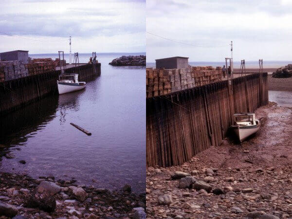
Display images showing high and low tide, such as those shown below:

Ask students:

• What do you notice about the water level in each image? 
• What do you think may have caused this change?

Step 2: BUILD KNOWLEDGE

• Read the description on the Tides topic page .
• Play the Movie , pausing to check for understanding. 
• Have students read one of the Related Reading articles. Partner them with someone who read a different article to share what they learned with each other.

Step 3: APPLY and ASSESS 

Students take the Tides Challenge and Quiz , applying essential literacy skills while demonstrating what they learned about this topic.

Step 4: EXTEND and DEEPEN

Students express what they learned about tides while practicing essential literacy skills with one or more of the following activities. Differentiate by assigning ones that meet individual student needs.

• Make-a-Movie : Produce a tutorial that answers this question: How can tides be an energy source?
• Make-a-Map : Create a concept map identifying the process that causes ocean levels to rise and fall.
• Creative Coding : Code a comic showing how types of tides can affect people visiting a beach.

More to Explore 

Related BrainPOP Topics : Deepen understanding of tides and related Earth systems with these topics: Gravity , Ocean Currents , Moon .

Teacher Support Resources:

• Learning Activities Modifications : Strategies to meet ELL and other instructional and student needs.
• Learning Activities Support : Resources for best practices using BrainPOP.

Lesson Plan Common Core State Standards Alignments

Lesson plan next generation science standards alignments.

• BrainPOP Jr. (K-3)
• BrainPOP ELL
• BrainPOP Science
• BrainPOP Español
• BrainPOP Français
• Set Up Accounts
• Single Sign-on
• Manage Subscription
• Quick Tours
• About BrainPOP

• Terms of Use
• Privacy Policy
• Trademarks & Copyrights

• Capital Campaign
• Mission Vision
• Racial Equity
• Staff and Board
• Open Positions
• In The News
• Past Newsletters
• Annual Reports
• Community Business Initiative
• In-Kind Support
• Partners & Supporters

Explore the Tides

Have you ever built a sandcastle on a beach only to find it washed away a few hours later? Every 6 to 12 hours or so, the water along most coasts rises and falls in a regular cycle called “tides.” What causes this phenomenon? In this lesson, students will apply what they know about gravity to the Sun-Earth-Moon system and to the occurrence of tides on Earth.

Objectives:

• Graph and analyze patterns in the times and heights of tides, moonrise and moonset times, and phases of the Moon along Virginia Beach.
• Build a model of the Earth-Moon system.
• Draw conclusions about the cause and occurrence of tides.
• Consider whether tidal processes exist on other planets and moons.
• Summarize and organize information about Pluto and compare Pluto to other planets.

Grade Level:

Estimated time:.

Depends on selected activities and class’ needs

Lesson Files

• Explore the Tides Lesson Plan (.pdf)
• Additional Tides Activity (.pdf)

Submit a Comment Cancel reply

Your email address will not be published. Required fields are marked *

Materials Needed for this Lesson Plan

• Tide Model Kit

Lesson Plans

Overview: Have you ever built a sandcastle on a beach only to find it washed away a few hours later? Every 6 to 12 hours or so, the water along most coasts rises and falls in...

Build an Electromagnet

Overview: Student teams investigate the properties of electromagnets. They create their own small electromagnets and experiment with ways to change their strength to pick up...

Tree Growth Study

Overview: How can the age of a tree be determined? Is there a way to tell a good year of growth versus a bad year? Trees contain some of nature’s most accurate records of...

Investigating Shadows

Overview: In this activity, students will explore what affects the size of a shadow and compare the shadows of various opaque, transparent, and translucent objects. Part I....

The Dirty Water Project

Overview: In this hands-on activity, students investigate different methods—aeration and filtering—for removing pollutants from water. Working in teams, they design,...

Drops on a Penny Experiment

Overview: Have you ever noticed on a rainy day how water forms droplets on a window? Why doesn’t it spread out evenly over the whole surface? It has to do with...

Modeling Gravity

Overview: Why can we feel gravity pull us down towards the Earth, but not sideways towards other big objects like buildings? Why do the planets in our solar system orbit the...

Floodplain Modeling

Overview: Students explore the impact of changing river volumes and different floodplain terrain in experimental trials with table top-sized riverbed models. The models are...

Build a Waterwheel from Recycled Materials

Overview: Students observe a model waterwheel to investigate the transformations of energy involved in turning the blades of a hydro-turbine. They work as engineers to create...

Entanglement Challenge

Demonstrate the challenges for marine animals who get entangled in common debris with this 10 –15 minute activity about marine conservation. Pair this activity with a...

Animal Yoga

Stretch your way into different animal movements and poses to learn how they move, get food, and protect themselves. This 5-10 minute full-body activity for young learners...

Weaving the Web of Life

Overview: In this hands-on activity, students construct a food web with yarn to learn how food chains are interconnected. Objectives: 1. construct a food chain and explain...

Battle of the Beaks: Adaptations and Niches

Overview: In this simulation game, students learn about adaptive advantage, based on beak function, by simulating birds competing for various foods. Birds equipped with...

Modeling the Seasons

This hands-on activity demonstrates and explains how seasons is caused by the tilt of Earth on its axis as it orbits around the sun. Students model the seasons with their...

Ring and Discs Demonstration

Ready, Set, Go! A ring and disc of equal mass and diameter speed down an inclined plane. Which one wins? Not an easy prediction to make, but the victor will be clear. Results...

Fire Syringe Demonstration

This is one of the most impressive demonstrations of the heat produced when a gas is rapidly compressed and is the principle behind how a diesel engine functions. How does it...

Repairing Broken Bones: Biomedical Engineering Design Challenge

This STEM activity incorporates the engineering design process into a life or biomedical science activity. It can be used during an anatomy unit or in a health...

Modeling Moon Phases

This lesson on the phases of the moon features just one of several hands-on activities you can do with our adaptable Moon Model Kit. In this activity students will: 1. use...

Color-Changing Celery Experiment

This exciting experiment illustrates transpiration, the process of plants absorbing water through their roots. The water travels up tubes in the stems called xylem to all...

10 Activities To Try With the Magnetic Water Molecules Kit

Try out 10 exciting activities related to the properties of matter using our Magnetic Water Molecules Kit! The following topics are covered: Polarity Hydrogen...

What's Your Blood Type?

Overview Realistically simulate blood typing without the hazards of real blood. Using actual blood typing procedures, students classify four unknown samples of the simulated...

Understanding Natural Selection Through Models

Overview With this worksheet, students will explore one of the five mechanisms of evolution: natural selection. Students will analyze and interpret 3 models of natural...

HIV/AIDS Test Simulation Lab

Explore the immunological principle that antibodies bind to specific antigens. Your class will learn how ELISA – Enzyme Linked Immunoassay – is a fundamental...

Egg in a Bottle

Overview: In this classic demonstration, students will use differences in air pressure to force an egg into a bottle. This demonstration only takes 10 minutes and leaves your...

Magnetic Meiosis Model Demonstration

Teach the mechanisms of meiosis (and make it memorable!) with this simple and informative magnetic demonstration. Instead of struggling to tell which chromosome is which from...

Modeling the Effects of an Introduced Species

Overview Using a set of Food Web cards, each depicting an organism, students work in groups to model a food web for one of four ecosystems. Students are then given an...

Natural Selection: Antibiotic Resistance and Engineering the Fastest Fish

Overview Immerse your students in this engaging 3-part laboratory activity on evolution by natural selection! Your students will practice important science skills while...

Estimating Populations

Background The size of an animal population becomes newsworthy when it becomes very large (too many rats in one place) or very small (on the verge of extinction). How do...

Butterfly Wings: Using Nature to Learn About Flight

Background Have you ever seen butterflies fluttering around outside, gliding through the air and landing on flowers? While they are delicate and fragile, butterflies are...

Osmosis and Diffusion Lab

This lab allows you to learn about two forms of passive transport: diffusion and osmosis. You will compare and contrast similarities and differences in the processes of...

Seed Identification Activity

This laboratory activity will familiarize students with basic plant anatomy and the basic characteristics and functions of plant seeds. Students will practice using...

Genetics: The Science of Heredity — Modeling DNA Structure and the Process of Replication

This lesson is the first unit of a 5 part module entitled “Genetics: The Science of Heredity” developed by ETA Cuisenaire. Modeling DNA structure and the process...

Crime Scene Investigation Lab

Innovating Science’s crime scene investigation lab is used to study forensic techniques and features an activity to solve the crime of the missing frogs from the...

Measuring Precipitation of Hurricanes

This lesson deepens students’ understanding of how and why we measure precipitation across the globe through the study of rainfall patterns caused by hurricanes. Students...

Prey vs. Predator

The action in this fast-paced activity may become intense as student “predators” attempt to capture their “prey.” What happens when different organisms, living in the...

What Is in the Food You Eat?

In this activity, students test representative food samples for the presence of certain types of matter (nutrients). This investigation allows students to discover some of...

The Science of Spherification

Forget drinking your juice. Instead, try snacking on it! Use the steps and recipes in this food science project to transform drinks into semi-solid balls that pop in your...

Turn Milk Into Plastic

“Plastic made from milk” —that certainly sounds like something made-up. If you agree, you may be surprised to learn that in the early 20th century, milk was...

Proper Hand Washing Can Stop the Spread of Disease

People used to believe that disease was caused by miasma, a poisonous vapor which carried particles of rotting materials that caused illness. People knew that eating spoiled...

How Germs Spread

People used to think that angry gods caused disease, or that a poisonous vapor that came from rotting food or bad air caused illness. It took thousands of years for people to...

7 Van De Graaff Generator Activities

A set of activities to show how the generator works and the principles behind it.

Calorimetry Lab

How does the energy content in lipids and carbohydrates differ? Energy content is the amount of heat produced by the burning of a small sample of a substance and heating...

Owl Pellet Surprise

This fun, hands-on introductory dissection is a great springboard for teaching the techniques of using a science notebook while having students engage in the...

Stream Table Investigation

Overview: Students learn about water erosion through an experimental process in which small-scale buildings are placed along a simulated riverbank to experience a range of...

Boiling by Pressure Drop

The goal of this experiment is to demonstrate that boiling is not just a function of temperature, as most people believe. Rather, it is a function of both temperature and...

How to Make Water Cycle in a Bag

https://www.mobileedproductions.com/blog/how-to-make-a-water-cycle-in-a-bag

How do Antibiotics Affect Bacteria When They are Put Together

Plan and carry out investigations: collaboratively, in a safe and ethical manner including personal impacts such as health safety, to produce data to serve as the basis...

Building a Generator

Students work individually or in pairs to follow a set of instructions and construct a mini generator which powers a Christmas light. Best done as a take-home assignment.

Conservation of Momentum with Vernier

Teacher leads a demonstration with vernier carts of different/equal mass, equipped with bumpers and magnets to demonstrate a variety of scenarios in which as both carts...

3rd Law with Vernier

After learning about the 1st law of motion, students partake in a teacher-led series of questions about 2 carts, and which cart will experience a greater force. The teacher...

Gravitational Acceleration

In 2-3 person groups, students take the mass of assorted objects, then hang them from a spring scale to find their gravitational force. Using the F=ma equation, they rewrite...

Electricity and Magnetism Stations

Egg drop lab.

Students work in teams to design a container for an egg using provided materials. Students drop their containers, then analyze factors which can minimize force on the...

How Does Volvo Keep Drivers Safe?

Students watch a series of short videos explaining how cars are designed with crumple zones, airbags, and automatic braking to prevent passenger damage in a collision....

Share Your Lesson Plan

We invite you to share your lesson plans as well so that we can continue to make this database a community resource.

• Name First Last
• Lesson Plan Name
• Description of Lesson
• Materials Borrowed for the Lesson
• Upload lesson plans, handouts, or other documents Drop files here or Accepted file types: pdf, doc, docx, xls, xlsx, ppt, pptx, pub, jpg, png.
• Name This field is for validation purposes and should be left unchanged.

OFFICE HOURS WITH EXPERTS

Connect with a local STEM professional or subject matter expert for help with specific content questions. Below is our current roster of subject matter experts.

Monica Pasos Audubon Nature Institute Biofacts and animals

Amanda Rosenzweig Delgado Community College Microscopes and microscopy

EARTH & ENVIRONMENTAL SCIENCE

Kyle Straub Tulane Local Louisiana ecology

LIFE SCIENCE

Physical science, robotics & engineering.

Cia Blackstock Director of Programs at Electric Girls Electrical engineering

STEM Library Lab is always looking for volunteers.

Whether you are a STEM practitioner and would like to become one of our local experts, a student looking to help with operations, or a member of the community interested in contributing to our mission in any way, we are eager to connect.

Just fill out the volunteer contact form and we’ll reach out soon!

• I am a... STEM professional or academic Teacher or school staff Student Community member Other
• I am interested in volunteering... At the library, assisting staff At the library, assisting teachers At a school Other
• Anything else you'd like us to know about your background or volunteer interests?
• Email This field is for validation purposes and should be left unchanged.

Our Location

3011 N I-10 Service Rd E Metairie LA 70002 504.517.3584

Note: we are no longer located on St Bernard Av.

Monday - Friday 2:00-5:00 p.m. And by appointment

• Nature of Inquiry Request inventory item Communities of practice Lesson plans Media inquiry Office hours with experts Microgrant opportunities Membership Sponsorship Other
• Your Inquiry

STEM Library Lab Membership

Thank you for your interest in becoming a member school. This form is for schools that want more information about the paid School Membership tier with additional member benefits.  Free membership is always free , simply create a borrower profile here .

Please complete the form below, and we'll be in touch quickly to learn more about you and your school.

• ROLE Role Principal Assistant Principal Teacher Teacher Aide Administrative Assistant Other
• HOW DID YOU HEAR ABOUT STEM LIBRARY LAB? Referral from Colleague Web Search Social Media
• Comments This field is for validation purposes and should be left unchanged.

Our monthly newsletter keeps you informed of goings-on, events, and high-interest items we stock.

• Community Member
• Phone This field is for validation purposes and should be left unchanged.
• Name * First Last
• School Name *
• Form Name / Title *
• Form Upload * Accepted file types: pdf, doc, docx, xls, xlsx, ppt, pptx, pub, jpg, png.
• Entry Form * Accepted file types: pdf, doc, docx, xls, xlsx, ppt, pptx, pub, jpg, png.
• Artwork * Accepted file types: pdf, doc, docx, xls, xlsx, ppt, pptx, pub, jpg, png.

Application Submission

• Project Title *
• Application Upload * Drop files here or Accepted file types: pdf, doc, docx, xls, xlsx, ppt, pptx, pub, jpg, png.

• school Campus Bookshelves
• menu_book Bookshelves
• perm_media Learning Objects
• login Login
• how_to_reg Request Instructor Account
• hub Instructor Commons
• Download Page (PDF)
• Download Full Book (PDF)
• Periodic Table
• Physics Constants
• Scientific Calculator
• Reference & Cite
• Tools expand_more
• Readability

selected template will load here

This action is not available.

7.6: Modeling with Trigonometric Equations

• Last updated
• Save as PDF
• Page ID 1372

Suppose we charted the average daily temperatures in New York City over the course of one year. We would expect to find the lowest temperatures in January and February and highest in July and August. This familiar cycle repeats year after year, and if we were to extend the graph over multiple years, it would resemble a periodic function.

Many other natural phenomena are also periodic. For example, the phases of the moon have a period of approximately 28 days, and birds know to fly south at about the same time each year. So how can we model an equation to reflect periodic behavior? First, we must collect and record data. We then find a function that resembles an observed pattern. Finally, we make the necessary alterations to the function to get a model that is dependable. In this section, we will take a deeper look at specific types of periodic behavior and model equations to fit data.

Determining the Amplitude and Period of a Sinusoidal Function

Any motion that repeats itself in a fixed time period is considered periodic motion and can be modeled by a sinusoidal function . The amplitude of a sinusoidal function is the distance from the midline to the maximum value, or from the midline to the minimum value. The midline is the average value. Sinusoidal functions oscillate above and below the midline, are periodic, and repeat values in set cycles. Recall from Graphs of the Sine and Cosine Functions that the period of the sine function and the cosine function is \(2π\). In other words, for any value of \(x\),

\[ \sin(x±2πk)=\sin x \; \text{and} \; \cos(x±2πk)=\cos x \]

where \(k\) is an integer.

STANDARD FORM OF SINUSOIDAL EQUATIONS

The general forms of a sinusoidal equation are given as

\[y=A \sin(Bt−C)+D\]

\[ y=A \cos(Bt−C)+D\]

where \(\text{amplitude}=|A|,B\) is related to period such that the \(\text{period}=\frac{2π}{B},C\) is the phase shift such that \(\frac{C}{B}\) denotes the horizontal shift, and \(D\) represents the vertical shift from the graph’s parent graph.

Note that the models are sometimes written as

\[y=a \sin (ω t±C)+D\]

\[y=a \cos(ω t±C)+D,\]

with a period that is given as \(\frac{2π}{ω}\).

The difference between the sine and the cosine graphs is that the sine graph begins with the average value of the function and the cosine graph begins with the maximum or minimum value of the function.

Example \(\PageIndex{1}\): Showing How the Properties of a Trigonometric Function Can Transform a Graph

Show the transformation of the graph of \(y=\sin x\) into the graph of \(y=2 \sin(4x−\frac{π}{2})+2\).

Consider the series of graphs in Figure \(\PageIndex{1}\) and the way each change to the equation changes the image.

• The basic graph of \(y=\sin x\)
• Changing the amplitude from 1 to 2 generates the graph of \(y=2 \sin x\).
• The period of the sine function changes with the value of \(B,\) such that \(\text{period}=\frac{2π}{B}.\) Here we have \(B=4,\) which translates to a period of \(\frac{π}{2}\). The graph completes one full cycle in \(\frac{π}{2}\) units.
• The graph displays a horizontal shift equal to \(\frac{C}{B}\), or \(\frac{\frac{π}{2}}{4}=\frac{π}{8}\).
• Finally, the graph is shifted vertically by the value of \(D\). In this case, the graph is shifted up by 2 units.

Example \(\PageIndex{2}\): Finding the Amplitude and Period of a Function

Find the amplitude and period of the following functions and graph one cycle.

• \(y=2 \sin (\frac{1}{4}x)\)
• \(y=−3 \sin (2x+\frac{π}{2})\)
• \(y= \cos x+3\)

We will solve these problems according to the models.

• \(y=2 \sin (\frac{1}{4}x)\) involves sine, so we use the form \[y=A \sin (Bt+C)+D \nonumber\] We know that \(| A |\) is the amplitude, so the amplitude is 2. Period is \(\frac{2π}{B}\) so the period is \[\begin{align*} \dfrac{2π}{B} &=\dfrac{2π}{\frac{1}{4}} \\ & =8π \end{align*}\] See the graph in Figure \(\PageIndex{3}\).

• \(y=−3 \sin(2x+ \frac{π}{2})\) involves sine, so we use the form \[y=A \sin (Bt−C)+D \nonumber\] Amplitude is \(| A |\), so the amplitude is \(|−3|=3.\) Since \(A\) is negative, the graph is reflected over the x -axis. Period is \(\frac{2π}{B}\),so the period is \[\dfrac{2π}{B}=\dfrac{2π}{2}=π \nonumber\] The graph is shifted to the left by \(\frac{C}{B}=\frac{\frac{π}{2}}{2}=\frac{π}{4}\) units. See Figure \(\PageIndex{4}\).

• \(y= \cos x+3\) involves cosine, so we use the form
• \[y=A \cos (Bt±C)+D \nonumber\] Amplitude is \(| A |\), so the amplitude is 1 and the period is \(2π\) (Figure \(\PageIndex{5}\). This is the standard cosine function shifted up three units.

Exercise \(\PageIndex{1}\):

What are the amplitude and period of the function \(y=3 \cos (3πx)\)?

The amplitude is \(3,\) and the period is \(\frac{2}{3}\).

Finding Equations and Graphing Sinusoidal Functions

One method of graphing sinusoidal functions is to find five key points. These points will correspond to intervals of equal length representing \(\frac{1}{4}\) of the period. The key points will indicate the location of maximum and minimum values. If there is no vertical shift, they will also indicate x -intercepts. For example, suppose we want to graph the function \(y=cos θ.\) We know that the period is \(2π\), so we find the interval between key points as follows.

\[\frac{2π}{4}=\frac{π}{2} \nonumber\]

Starting with \(θ=0,\) we calculate the first y- value, add the length of the interval \(\frac{π}{2}\) to \(0\), and calculate the second y -value. We then add \(\frac{π}{2}\) repeatedly until the five key points are determined. The last value should equal the first value, as the calculations cover one full period. Making a table similar to Table \(\PageIndex{1}\), we can see these key points clearly on the graph shown in Figure \(\PageIndex{6}\).

Example \(\PageIndex{3}\): Graphing Sinusoidal Functions Using Key Points

Graph the function \(y=−4 \cos (πx)\) using amplitude, period, and key points.

The amplitude is \(|−4|=4.\) The period is \(\frac{2π}{ω}=\frac{2π}{π}=2.\) (Recall that we sometimes refer to \(B\) as \(ω.\)) One cycle of the graph can be drawn over the interval \([ 0,2 ]\). To find the key points, we divide the period by 4. Make a table similar to Figure \(\PageIndex{1}\):, starting with \(x=0\) and then adding \(\frac{1}{2}\) successively to \(x\) and calculate \(y.\) See the graph in Figure \(\PageIndex{7}\).

Exercise \(\PageIndex{2}\):

Graph the function \(y=3 \sin(3x)\) using the amplitude, period, and five key points.

Modeling Periodic Behavior

We will now apply these ideas to problems involving periodic behavior.

Example \(\PageIndex{4}\): Modeling an Equation and Sketching a Sinusoidal Graph to Fit Criteria

The average monthly temperatures for a small town in Oregon are given in Table \(\PageIndex{1}\). Find a sinusoidal function of the form \(y=A \sin (Bt−C)+D\) that fits the data (round to the nearest tenth) and sketch the graph.

Recall that amplitude is found using the formula

\[A=\dfrac{\text{largest value −smallest value}}{2}\]

Thus, the amplitude is

\[\begin{align*} |A| & = \dfrac{69−42.5}{2} \\ &=13.25 \end{align*}\]

The data covers a period of 12 months, so \(\frac{2π}{B}=12\) which gives \(B=\frac{2π}{12}=\frac{π}{6}\).

The vertical shift is found using the following equation.

\[D=\dfrac{\text{highest value+lowest value}}{2}\]

\[\begin{align*} D &= \dfrac{69+42.5}{2} &=55.8 \end{align*}\]

So far, we have the equation \(y=13.3 \sin (\frac{π}{6}x−C)+55.8\).

To find the horizontal shift, we input the \(x\) and \(y\) values for the first month and solve for \(C\).

\[\begin{align*} 42.5 & =13.3 \sin (\frac{π}{6}(1)−C)+55.8 \\ −13.3 & =13.3 \sin (\frac{π}{6}−C) \\ −1 & =\sin (\frac{π}{6}−C) \;\;\;\;\;\;\;\; \sin θ=−1→ θ=−\frac{π}{2} \\ \frac{π}{6}−C=−\frac{π}{2} \\ \frac{π}{6}+\frac{π}{2} & =C \\ &=\frac{2π}{3} \end{align*}\]

We have the equation \(y=13.3 \sin (\frac{π}{6}x−\frac{2π}{3})+55.8\). See the graph in Figure \(\PageIndex{9}\).

Example \(\PageIndex{5}\): Describing Periodic Motion

The hour hand of the large clock on the wall in Union Station measures 24 inches in length. At noon, the tip of the hour hand is 30 inches from the ceiling. At 3 PM, the tip is 54 inches from the ceiling, and at 6 PM, 78 inches. At 9 PM, it is again 54 inches from the ceiling, and at midnight, the tip of the hour hand returns to its original position 30 inches from the ceiling. Let \(y\) equal the distance from the tip of the hour hand to the ceiling \(x\) hours after noon. Find the equation that models the motion of the clock and sketch the graph.

Begin by making a table of values as shown in Table \(\PageIndex{3}\).

To model an equation, we first need to find the amplitude.

\[\begin{align*} | A | & =| \dfrac{78−30}{2} | \\ &=24 \end{align*}\]

The clock’s cycle repeats every 12 hours. Thus,

\[\begin{align*} B &=\dfrac{2π}{12} \\ &= \dfrac{π}{6} \end{align*}\]

The vertical shift is

\[\begin{align*} D & = \dfrac{78+30}{2} \\ &=54 \end{align*}\]

There is no horizontal shift, so \(C=0.\) Since the function begins with the minimum value of \(y\) when \(x=0\) (as opposed to the maximum value), we will use the cosine function with the negative value for \(A\). In the form \(y=A \cos (Bx±C)+D,\) the equation is

\[y=−24 \cos (\dfrac{π}{6}x)+54\]

See Figure \(\PageIndex{10}\).

Example \(\PageIndex{6}\): Determining a Model for Tides

The height of the tide in a small beach town is measured along a seawall. Water levels oscillate between 7 feet at low tide and 15 feet at high tide. On a particular day, low tide occurred at 6 AM and high tide occurred at noon. Approximately every 12 hours, the cycle repeats. Find an equation to model the water levels.

As the water level varies from 7 ft to 15 ft, we can calculate the amplitude as

\[ \begin{align*} |A| &=| \frac{(15−7)}{2} | \\ & =4 \end{align*}\]

The cycle repeats every 12 hours; therefore, \(B\) is

\[\begin{align*} \dfrac{2π}{12}=\dfrac{π}{6} \end{align*}\]

There is a vertical translation of \(\frac{(15+8)}{2}=11.5\). Since the value of the function is at a maximum at \(t=0\), we will use the cosine function, with the positive value for \(A\).

\[y=4 \cos (\dfrac{π}{6}) t+11 \nonumber\]

See Figure \(\PageIndex{11}\).

Exercise \(\PageIndex{3}\):

The daily temperature in the month of March in a certain city varies from a low of \(24°F\) to a high of \(40°F.\) Find a sinusoidal function to model daily temperature and sketch the graph. Approximate the time when the temperature reaches the freezing point \(32 °F.\) Let \(t=0\) correspond to noon.

\[y=8 \sin (\frac{π}{12}t)+32 \nonumber\]

Exercise \(\PageIndex{4}\): Interpreting the Periodic Behavior Equation

The average person’s blood pressure is modeled by the function \(f(t)=20 \sin (160πt)+100\), where \(f(t)\) represents the blood pressure at time \(t\), measured in minutes. Interpret the function in terms of period and frequency. Sketch the graph and find the blood pressure reading.

Blood pressure of \(\frac{120}{80}\) is considered to be normal. The top number is the maximum or systolic reading, which measures the pressure in the arteries when the heart contracts. The bottom number is the minimum or diastolic reading, which measures the pressure in the arteries as the heart relaxes between beats, refilling with blood. Thus, normal blood pressure can be modeled by a periodic function with a maximum of 120 and a minimum of 80.

Example \(\PageIndex{7}\): Interpreting the Periodic Behavior Equation

The period is given by

\[\begin{align*} \dfrac{2π}{ω} & = \dfrac{2π}{160π} \\ &=\dfrac{1}{80} \end{align*}\]

In a blood pressure function, frequency represents the number of heart beats per minute. Frequency is the reciprocal of period and is given by

\[\begin{align*} \dfrac{ω}{2π} & = \dfrac{160π}{2π} \\ & =80 \end{align*}\]

Modeling Harmonic Motion Functions

Harmonic motion is a form of periodic motion, but there are factors to consider that differentiate the two types. While general periodic motion applications cycle through their periods with no outside interference, harmonic motion requires a restoring force. Examples of harmonic motion include springs, gravitational force, and magnetic force.

Simple Harmonic Motion

A type of motion described as simple harmonic motion involves a restoring force but assumes that the motion will continue forever. Imagine a weighted object hanging on a spring, When that object is not disturbed, we say that the object is at rest, or in equilibrium. If the object is pulled down and then released, the force of the spring pulls the object back toward equilibrium and harmonic motion begins. The restoring force is directly proportional to the displacement of the object from its equilibrium point. When \(t=0,d=0.\)

SIMPLE HARMONIC MOTION

We see that simple harmonic motion equations are given in terms of displacement:

\[d=a \cos (ωt) \; \text{or} \; d=a \sin (ωt) \]

where \(| a |\) is the amplitude, \(\frac{2π}{ω}\) is the period, and \(\frac{ω}{2π}\) is the frequency, or the number of cycles per unit of time.

Exercise \(\PageIndex{5}\): Finding the Displacement, Period, and Frequency, and Graphing a Function

For each the given functions:

• \(y=5 \sin (3t)\)
• \(y=6 \cos (πt)\)
• \(y=5 \cos (\frac{π}{2}) t\)

address the following questions:

• Find the maximum displacement of an object.
• Find the period or the time required for one vibration.
• Find the frequency.
• Sketch the graph.

• The maximum displacement is equal to the amplitude,\( |a|\), which is 5.
• The period is \(\frac{2π}{ω}=\frac{2π}{3}\).
• The frequency is given as \(\frac{ω}{2π}=\frac{3}{2π}\).
• See Figure \(\PageIndex{13}\). The graph indicates the five key points.
• The maximum displacement is \(6\).
• The period is \(\frac{2π}{ω}=\frac{2π}{π}=2.\)
• The frequency is \(\frac{ω}{2π}=\frac{π}{2π}=\frac{1}{2}.\)
• See Figure \(\PageIndex{14}\).

• The maximum displacement is \(5\).
• The period is \(\frac{2π}{ω}=\frac{2π}{\frac{π}{2}}=4\).
• The frequency is \(\frac{1}{4}.\)
• See Figure \(\PageIndex{15}\).

Damped Harmonic Motion

In reality, a pendulum does not swing back and forth forever, nor does an object on a spring bounce up and down forever. Eventually, the pendulum stops swinging and the object stops bouncing and both return to equilibrium. Periodic motion in which an energy-dissipating force, or damping factor, acts is known as damped harmonic motion . Friction is typically the damping factor.

In physics, various formulas are used to account for the damping factor on the moving object. Some of these are calculus-based formulas that involve derivatives. For our purposes, we will use formulas for basic damped harmonic motion models.

Definition: DAMPED HARMONIC MOTION

In damped harmonic motion , the displacement of an oscillating object from its rest position at time \(t\) is given as

\[ f(t)=ae^{−ct} \sin (ωt) \; \text{ or} \; f(t)=ae^{−ct} \cos (ωt)\]

where \(c\) is a damping factor, \(|a|\) is the initial displacement and \(\frac{2π}{ω}\) is the period.

Example \(\PageIndex{8}\): Modeling Damped Harmonic Motion

Model the equations that fit the two scenarios and use a graphing utility to graph the functions: Two mass-spring systems exhibit damped harmonic motion at a frequency of 0.5 cycles per second. Both have an initial displacement of 10 cm. The first has a damping factor of 0.5 and the second has a damping factor of 0.1.

At time \(t=0\), the displacement is the maximum of 10 cm, which calls for the cosine function. The cosine function will apply to both models.

We are given the frequency \(f=\frac{ω}{2π}\) of 0.5 cycles per second. Thus,

\[\begin{align*} \dfrac{ω}{2π} &=0.5 \\ ω&=(0.5)2π \\ &=π \end{align*}\]

The first spring system has a damping factor of \(c=0.5\). Following the general model for damped harmonic motion, we have

\[f(t)=10e^{−0.5t} \cos (πt) \nonumber\]

Figure \(\PageIndex{16}\) models the motion of the first spring system.

The second spring system has a damping factor of \(c=0.1\) and can be modeled as

\[f(t)=10e^{−0.1t} \cos (πt)\]

Figure \(\PageIndex{17}\) models the motion of the second spring system.

Notice the differing effects of the damping constant. The local maximum and minimum values of the function with the damping factor \(c=0.5\) decreases much more rapidly than that of the function with \(c=0.1\).

Exercise \(\PageIndex{6}\): Finding a Cosine Function that Models Damped Harmonic Motion

Find and graph a function of the form \(y=ae^{−ct} \cos (ωt)\) that models the information given.

• \(a=20,c=0.05,p=4\)
• \(a=2,c=1.5,f=3\)

Substitute the given values into the model. Recall that period is \(\frac{2π}{ω}\) and frequency is \(\frac{ω}{2π}\).

Exercise \(\PageIndex{7}\)

The following equation represents a damped harmonic motion model: \(f(t)=5e^{−6t} \cos (4t)\) Find the initial displacement, the damping constant, and the frequency.

initial displacement =6, damping constant = -6, frequency =\(\frac{2}{π}\)

Example \(\PageIndex{9}\): Finding a Sine Function that Models Damped Harmonic Motion

Find and graph a function of the form \(y=ae^{−ct} \sin (ωt)\) that models the information given.

• \(a=7,c=10,p=\frac{π}{6}\)
• \(a=0.3,c=0.2,f=20\)

Calculate the value of \(ω\) and substitute the known values into the model.

\[\begin{align*} \dfrac{π}{6} &=\dfrac{2π}{ω} \\ ωπ &=6(2π) \\ ω &=12 \end{align*}\]

The damping factor is given as 10 and the amplitude is 7. Thus, the model is \(y=7e^{−10t} \sin (12t)\). See Figure \(\PageIndex{20}\).

\[\begin{align*} 20 &=\dfrac{ω}{2π} \\ 40π &=ω \end{align*}\]

The damping factor is given as \(0.2\) and the amplitude is \(0.3.\) The model is \(y=0.3e^{−0.2t} \sin (40πt).\) See Figure \(\PageIndex{21}\).

A comparison of the last two examples illustrates how we choose between the sine or cosine functions to model sinusoidal criteria. We see that the cosine function is at the maximum displacement when \(t=0\), and the sine function is at the equilibrium point when \(t=0.\) For example, consider the equation \(y=20e^{−0.05t} \cos (\frac{π}{2}t)\) from Example. We can see from the graph that when \(t=0,y=20,\) which is the initial amplitude. Check this by setting \(t=0\) in the cosine equation:

\[ \begin{align*} y &=20e^{−0.05(0)} \cos (\frac{π}{2})(0) \\ &=20(1)(1) \\ & =20 \end{align*}\]

Using the sine function yields

\[\begin{align*} y &=20e^{−0.05(0)} \sin (\frac{π}{2})(0) \\ & =20(1)(0) \\ &=0 \end{align*}\]

Thus, cosine is the correct function.

Exercise \(\PageIndex{8}\):

Write the equation for damped harmonic motion given \(a=10,c=0.5\), and \(p=2.\)

\(y=10e^{−0.5t} \cos (πt)\)

Example \(\PageIndex{10}\): Modeling the Oscillation of a Spring

A spring measuring 10 inches in natural length is compressed by 5 inches and released. It oscillates once every 3 seconds, and its amplitude decreases by 30% every second. Find an equation that models the position of the spring \(t\) seconds after being released.

The amplitude begins at 5 in. and deceases 30% each second. Because the spring is initially compressed, we will write A as a negative value. We can write the amplitude portion of the function as

\[A(t)=5(1−0.30)^t \nonumber\]

We put \((1−0.30)^t\) in the form \(e^{ct}\) as follows:

\[\begin{align*} 0.7 &=e^c \\ c &= \ln .7 \\ c & =−0.357 \end{align*}\]

Now let’s address the period. The spring cycles through its positions every 3 seconds, this is the period, and we can use the formula to find omega.

\[\begin{align*} 3 &= \dfrac{2π}{ω} \\ ω &= \dfrac{2π}{3} \end{align*}\]

The natural length of 10 inches is the midline. We will use the cosine function, since the spring starts out at its maximum displacement. This portion of the equation is represented as

\[y=\cos (\dfrac{2π}{3}t)+10 \nonumber\]

Finally, we put both functions together. Our the model for the position of the spring at \(t\) seconds is given as

\[y=−5e^{−0.357t} \cos (\dfrac{2π}{3}t)+10 \nonumber\]

See the graph in Figure \(\PageIndex{22}\).

Exercise \(\PageIndex{9}\)

A mass suspended from a spring is raised a distance of 5 cm above its resting position. The mass is released at time \(t=0\) and allowed to oscillate. After \(\frac{1}{3}\) second, it is observed that the mass returns to its highest position. Find a function to model this motion relative to its initial resting position.

\(y=5 \cos (6πt)\)

According to the Given Criteria

A guitar string is plucked and vibrates in damped harmonic motion. The string is pulled and displaced 2 cm from its resting position. After 3 seconds, the displacement of the string measures 1 cm. Find the damping constant.

The displacement factor represents the amplitude and is determined by the coefficient \(ae^{−ct}\) in the model for damped harmonic motion. The damping constant is included in the term \(e^{−ct}\). It is known that after 3 seconds, the local maximum measures one-half of its original value. Therefore, we have the equation

\[ae^{−c(t+3)}=\dfrac{1}{2} ae^{−ct}\]

Use algebra and the laws of exponents to solve for \(c\).

\[\begin{array}{cl} ae^{−c(t+3)}=\frac{1}{2}ae^{−ct} \\ e^{−ct}⋅e^{−3c}=\frac{1}{2}e^{−ct} & \text{Divide out } a. \\ e^{−3c}=\frac{1}{2} & \text{Divide out }e^{−ct}. \\ e^{3c}=2 & \text{Take reciprocals.} \end{array}\]

Then use the laws of logarithms.

\[\begin{align*} e^{3c} &=2 \\ 3c &=\ln 2 \\ c & =\frac{\ln 2}{3} \end{align*}\]

The damping constant is \(\frac{\ln 2}{3}\).

Bounding Curves in Harmonic Motion

Harmonic motion graphs may be enclosed by bounding curves. When a function has a varying amplitude , such that the amplitude rises and falls multiple times within a period, we can determine the bounding curves from part of the function.

Example \(\PageIndex{12}\): Graphing an Oscillating Cosine Curve

Graph the function \(f(x)=\cos (2πx) \cos (16πx)\).

The graph produced by this function will be shown in two parts. The first graph will be the exact function \(f(x)\) (see Figure \(\PageIndex{23; top}\);), and the second graph is the exact function \(f(x)\) plus a bounding function (see Figure \(\PageIndex{23; bottom}\)). The graphs look quite different.

Figure \(\PageIndex{23}\)

The curves \(y=\cos (2πx)\) and \(y=−\cos (2πx)\) are bounding curves: they bound the function from above and below, tracing out the high and low points. The harmonic motion graph sits inside the bounding curves. This is an example of a function whose amplitude not only decreases with time, but actually increases and decreases multiple times within a period.

Key Equations

Key concepts.

• Sinusoidal functions are represented by the sine and cosine graphs. In standard form, we can find the amplitude, period, and horizontal and vertical shifts. See Example and Example.
• Use key points to graph a sinusoidal function. The five key points include the minimum and maximum values and the midline values. See Example.
• Periodic functions can model events that reoccur in set cycles, like the phases of the moon, the hands on a clock, and the seasons in a year. See Example, Example, Example and Example.
• Harmonic motion functions are modeled from given data. Similar to periodic motion applications, harmonic motion requires a restoring force. Examples include gravitational force and spring motion activated by weight. See Example.
• Damped harmonic motion is a form of periodic behavior affected by a damping factor. Energy dissipating factors, like friction, cause the displacement of the object to shrink. See Example, Example, Example, Example, and Example.
• Bounding curves delineate the graph of harmonic motion with variable maximum and minimum values. See Example.