case study in excel

Table of Contents

Data Analysis Using Excel Case Study

Data analysis is an essential skill in today’s business world. As organizations deal with increasing amounts of data, it becomes crucial for professionals to make sense of this information and derive useful insights. Excel is a powerful and versatile tool that can assist in analyzing and presenting data effectively, particularly through the use of case studies.

A case study is a detailed examination of a specific situation or problem in order to better understand the complexities involved. By using Excel for data analysis, individuals can explore and analyze the data related to the case study in a comprehensive and structured manner. Excel offers various tools and functionalities, such as PivotTables, slicers, and data visualization features, which allow users to assess patterns, trends, and relationships within the data.

Applying these techniques for data analysis in Excel case studies enables professionals to make well-informed business decisions and communicate their findings effectively. By leveraging the capabilities of Excel in conjunction with case studies, individuals can unlock valuable insights that drive organizational success and contribute to an enhanced understanding of the overall data landscape.

Excel Basics for Data Analysis

Dataset preparation.

When working with Excel, the first step in data analysis is dataset preparation . This process involves setting up the data in a structured format, with clearly defined headers and cells. To start, you must import or enter your data into an Excel spreadsheet, ensuring that each record is represented by a row and each variable by a column. Headers should be placed in the top row and provide descriptive labels for each column. Proper organization of your dataset helps to ensure accurate analysis and interpretation .

For example, suppose you have a dataset that contains the following information:

In this dataset, the headers are “Year,” “Category,” “Sales,” and “Profit.” Each row represents a record, and the cells contain the corresponding data.

Data Cleaning

The next step in data analysis using Excel is data cleaning . Data cleaning is the process of identifying and correcting errors, inconsistencies, and inaccuracies in your dataset. Common data cleaning tasks include:

• Removing duplicate records,
• Filling in missing values,
• Correcting data entry errors,
• Standardizing and formatting variable names and values.

To perform data cleaning in Excel, you can use various functions and tools:

• Remove duplicates: To remove duplicate records, select your dataset and navigate to the Data tab. Click the “Remove Duplicates” button and select the columns to be used for identifying duplicate rows.
• Fill in missing values: Use Excel functions such as VLOOKUP , HLOOKUP , and INDEX-MATCH to fill in missing values based on other data in your dataset. You can also use the IFERROR function to handle errors when looking up values.
• Correct data entry errors: Use Excel’s “Find and Replace” tool (Ctrl + F) to search for and correct errors in your dataset. You may need to perform this multiple times for different errors.
• Standardize and format variable names and values: Use Excel functions such as UPPER , LOWER , PROPER , and TRIM to standardize text data. Format numerical values using the Number Format options in the Home tab.

By ensuring your dataset is clean and well-organized, you can confidently move forward with more advanced data analysis tasks in Excel.

Powerful Excel Functions

Excel is a versatile tool when it comes to data analysis. There are many powerful functions that can help you perform complex calculations and analysis easily. In this section, we will explore some of the top functions in three categories: Text Functions, Date Functions, and Lookup Functions.

Text Functions

Text Functions are crucial when working with large sets of data containing text. These functions help in cleaning, extracting, and modifying text data. Some key text functions include:

• LEFT : Extracts a specified number of characters from the beginning of a text string.
• RIGHT : Extracts a specified number of characters from the end of a text string.
• MID : Extracts a specified number of characters from a text string, starting at a specified position.
• TRIM : Removes extra spaces from text, leaving a single space between words and no space at the beginning or end of the text.
• CONCATENATE : Joins multiple text strings into one single string.
• FIND : Locates the position of a specific character or text string within another text string.

Date Functions

Date Functions are essential for dealing with dates and times in data analysis. These functions help in calculating the difference between dates, extracting parts of a date, and performing various date-related calculations. Some notable date functions include:

• TODAY : Returns the current date.
• NOW : Returns the current date and time.
• DATEDIF : Calculates the difference between two dates in days, months, or years.
• DATE : Creates a date by combining individual day, month, and year values.
• WEEKDAY : Returns the day of the week corresponding to a specific date, as an integer between 1 (Sunday) and 7 (Saturday).
• EOMONTH : Returns the last day of the month for a given date.

Lookup Functions

Lookup Functions are powerful tools used to search and retrieve data from a specific range or table in Excel. These functions can save time and effort when working with large datasets. Some essential lookup functions include:

• VLOOKUP : Searches for a specific value in the first column of a range and returns a corresponding value from a specified column.
• HLOOKUP : Searches for a specific value in the first row of a range and returns a corresponding value from a specified row.
• INDEX : Returns a value from a specific cell within a range, using row and column numbers.
• MATCH : Searches for a specific value in a range and returns its relative position within that range.
• XLOOKUP : Performs a lookup by searching for a specific value in a range or table and returning a corresponding value from another column or row (available only in Excel 365 and Excel 2019).

These powerful Excel functions can help make the process of data analysis more efficient and accurate. In combination with appropriate formatting, tables, and other visual aids, these functions can greatly enhance your ability to process and understand large datasets.

Related Article: Excel Functions for Data Analysts.

Data Exploration and Visualization

In the process of data analysis using Excel, data exploration and visualization play essential roles in revealing patterns, trends, and relationships within the data. This section will cover two primary techniques for data visualization in Excel: Charts and Trends, and Pivot Tables and Pivot Charts.

Charts and Trends

Charts in Excel are a highly effective method of uncovering patterns and relationships within the dataset. There are various types of charts available in Excel that cater to different use cases, such as bar charts, line charts, and scatter plots. These chart types can be customized to suit the needs of the analysis and to emphasize specific trends or patterns.

Trends in the data can be identified with the help of charts, and Excel offers trend lines functionalities to visualize these trends more clearly. By applying a trend line, one can easily identify the overall direction (positive or negative) of the dataset and make predictions based on this information. Additionally, Excel offers built-in formatting options that can help emphasize certain data points or highlight particular trends for easier interpretation.

Pivot Tables and Pivot Charts

Pivot Tables are another powerful data analysis feature in Excel. They allow the user to summarize, reorganize, and filter data by dragging and dropping columns into different areas. This enables the user to analyze data across multiple dimensions, revealing hidden insights and patterns.

To complement Pivot Tables, Excel also offers Pivot Charts, which allow users to create dynamic visualizations derived from the Pivot Table data. Pivot Charts offer the same chart types as regular Excel charts but with the added capability to update the chart when the Pivot Table data is altered. This makes Pivot Charts ideal for creating interactive and easily updatable visualizations.

Overall, incorporating these techniques into the data analysis process can enhance understanding and unveil valuable insights from the dataset. When using Excel for data analysis, data exploration and visualization with Charts and Trends, as well as Pivot Tables and Pivot Charts, can provide a comprehensive and insightful overview of the data in question.

Case Study: Covid-19 Data Analysis

Data collection and cleaning.

The Covid-19 pandemic has generated vast amounts of data, requiring researchers and analysts to collect, clean, and organize data sets to gain valuable insights. Several sources, such as the World Health Organization and Johns Hopkins University , provide updated information on confirmed cases, recoveries, and deaths.

Data collection starts with gathering raw data from various sources. These data sets may have inconsistencies, missing values, or discrepancies, which need to be addressed to ensure accurate analysis. Data cleaning is a critical step in this process, involving tasks such as removing duplicates, filling in missing values, and correcting errors.

Exploratory Data Analysis

Once the data is clean and organized, exploratory data analysis (EDA) can be conducted using tools like Excel. EDA helps analysts understand the data, identify patterns, and generate hypotheses for further investigation.

Some useful techniques in conducting EDA in Excel include:

• Pivot Tables : These allow users to summarize and reorganize data quickly, providing aggregated views of the data.
• Charts and Graphs : Visual representations of data, such as bar charts or line graphs, can display trends, correlations, or patterns more clearly than raw numbers.
• Descriptive Statistics : Excel’s built-in functions allow easy calculation of measures such as mean, median, and standard deviation, providing a preliminary statistical analysis of the data.

In the context of Covid-19 data, EDA can help reveal important information about the pandemic’s progression. For example, analysts can:

• Compare infection rates across countries or regions
• Monitor changes in case numbers over time
• Evaluate the effectiveness of public health interventions and policies

The insights gained from exploratory data analysis can guide further research, inform decision-making, and contribute to a better understanding of the pandemic’s impact on public health.

Case Study: Stock Market Data Analysis

Data collection and preparation.

The first step in the stock market data analysis case study is collecting and preparing the data. This process involves gathering historical stock prices, trading volumes, and other relevant financial metrics from reliable sources. The data can be cleaned and organized in Excel, removing any errors or inconsistencies. It’s essential to verify the collected data’s accuracy to ensure the analysis’s validity.

After preparing the financial data, the next step is to compute essential measures and ratios. These may include:

• Price-to-Earnings (P/E) Ratio
• Dividends Yield
• Total Return
• Moving Averages

Calculating these ratios and measures provides a general overview of a company’s performance in the stock market, which can be further analyzed with Excel tools.

Profit and Loss Analysis

In this stage of the case study, profit and loss analysis is conducted to assess the stock’s performance. Using Excel PivotTables, we can summarize the data to identify trends or patterns in the stock market. For instance, we can analyze the historical profits and losses of multiple stocks during a specific state or market condition.

Analyzing profit and loss data can also be done with natural language capabilities in Excel. This feature allows us to ask questions about the dataset, and Excel will produce relevant results. For example, we could pose a question like “Which stocks had the highest profit margins in the last quarter?” or “What is the average loss for the technology sector?”

After exploring the profits and losses of the stocks, we can gain insights into which stocks or sectors are more profitable or risky. This information can help potential investors make informed decisions about their investment strategies. Additionally, the insights from the case study can serve as a reference point for future stock market analyses.

Remember, this case study only serves as an example of how to conduct stock market data analysis using Excel. By adapting and expanding on these techniques, one can harness the power of Excel to explore various aspects of financial markets and derive valuable insights.

Case Study: San Diego Burrito Ratings

Data gathering and cleaning.

The main objective of this case study is to evaluate and analyze the various factors that contribute to the ratings of San Diego burritos. The data used in this analysis is collected from different sources, which include customer reviews and ratings from Yelp, along with other relevant information about burrito sales and geographical distribution. The raw data is then compiled and cleaned to ensure that it is consistent and free from any discrepancies or errors. This process involves standardizing the fields and records, as well as filtering out any irrelevant information. The cleaned data is then organized into a structured format, which is suitable for further analysis using Excel PivotTables and Charts.

Use of Pivot Tables and Charts

After cleaning and organizing the data, Excel PivotTables are utilized to analyze the regional distribution of San Diego burrito ratings. By categorizing the data based on regions, such as East and West, it becomes convenient to identify the ratings and sales trends across these regions. The organized data is then sorted based on the ratings and popularity of burrito establishments within specific densely populated areas.

Using Pivot Charts, a graphical representation of the data is created to provide a clear and comprehensive visual of the ratings distribution in different regions of San Diego. It becomes easier to discern patterns and trends, allowing for the development of informed conclusions on the factors influencing the popularity and success of burrito establishments.

Throughout the analysis, various parameters are investigated, which include the relationship between ratings and sales, the potential impact of particular fields on popularity, and the apparent differences between densely populated regions in terms of burrito preferences. By utilizing PivotTables and Charts confidently, it is possible to draw insights and conclusions that can help optimize marketing strategies, guide customer preferences, and influence the overall success of burrito establishments across San Diego.

Case Study: Shark Attack Records Analysis

Data collection and pre-processing.

In this case study, the primary focus is on the analysis of shark attack records recorded between 1900 and 2016, consisting of just under 5,300 records or observations. To begin the analysis, the data needs to be collected from a reliable source and pre-processed to ensure its accuracy and relevance.

Data pre-processing is an essential step to prepare the dataset for analysis. It involves checking for missing values, outliers, and inconsistencies in the data. Additionally, it may also require converting the data into a suitable format, such as categorizing dates or splitting location information into separate columns (latitude and longitude).

Identifying Trends and Patterns

Once the dataset has been pre-processed, it’s time to dive into the analysis using Microsoft Excel. Excel offers a fast and central way to analyze data and search for trends and patterns within shark attack records. One powerful tool for this purpose is Excel’s PivotTables, which allows users to easily aggregate and summarize data.

Some possible trends and patterns that can be identified through the analysis of shark attack records include:

• Temporal Trends: Analyzing the frequency of shark attacks over time to identify any patterns in the occurrence of attacks, such as seasonality or specific years with higher attack rates.
• Geographical Patterns: Identifying areas with a higher concentration of shark attacks, which can provide insights into hotspots and potentially dangerous locations.
• Victim Demographics: Examining the demographics of shark attack victims, such as age, gender, and activity type, to determine if certain groups are more prone to attacks.
• Species Involved: Investigating the types of shark species responsible for attacks and their relative frequency in the dataset.

By utilizing Excel’s data analysis tools and PivotTables, researchers can confidently and clearly identify trends and patterns in the shark attack records, providing valuable insights into shark behavior and risk factors associated with shark attacks. This analysis can be helpful in understanding and managing the risks associated with shark encounters for both public safety and conservation efforts.

Related Article: How to Solve Data Analysis Real World Problems.

Additional Resources and Exercises

Kaggle and data analysis courses.

Kaggle is a popular platform that offers data science competitions, datasets, and courses to help you improve your data analysis skills in Excel. The courses are designed for various skill levels, and they cover essential concepts like PivotTables and data visualization. The comprehensive exercises and practical case studies provide a real-world context for mastering data analysis techniques.

The course reviews on Kaggle are usually quite positive, with many users appreciating the knowledgeable instructors and engaging content. If you’re looking to become a data analyst or enhance your existing skills, exploring the data analysis courses on Kaggle is a great starting point.

Power Query in Excel

Power Query is a powerful data analysis tool in Excel that enables you to import, transform, and combine data from various sources. This feature is particularly useful when working with large datasets or preparing data for analysis. There are numerous resources available to learn how to use Power Query effectively.

To practice using Power Query, consider working on exercises that focus on data cleansing, data transformation, and data integration. As you progress, you will gain a deeper understanding of the various Power Query functionalities and become more confident in your data analysis abilities.

In conclusion, engaging with additional resources like Kaggle courses and Power Query exercises will help you hone your Excel data analysis skills and enable you to tackle complex case studies with ease.

Frequently Asked Questions

How can excel be used for effective case study analysis.

Excel is a versatile tool that can be utilized for effective case study analysis. By organizing and transforming data into easily digestible formats, users can better identify trends, patterns, and insights within their data sets. Excel also offers various functions and tools, such as pivot tables, data tables, and data visualization, which enable users to analyze case study data more efficiently and uncover valuable information.

Which Excel functions are most useful for data analysis in case studies?

There are numerous Excel functions that can be highly useful for data analysis in case studies. These include:

• VLOOKUP, which allows users to search for specific information in large data sets
• INDEX-MATCH, a more advanced alternative to VLOOKUP that’s capable of handling more complex data structures
• IF, which helps in making conditional statements and decisions in data analysis
• AVERAGE, MAX, MIN, and COUNT for basic data aggregation
• SUMIFS and COUNTIFS, which allow users to perform conditional aggregation based on predefined criteria

What are some examples of data analysis projects using Excel?

Many different projects can benefit from data analysis using Excel, such as financial analysis, market research, sales performance tracking, and customer behavior analysis. Businesses across industries are known to use Excel for evaluating their case studies and forming data-driven decisions based on their insights.

How can Excel pivot tables aid in analyzing case study data?

Pivot tables in Excel are powerful, enabling users to summarize and analyze large data sets quickly and efficiently. They allow users to group and filter data based on different dimensions, making it much easier to identify trends, patterns, and relationships within the data. Additionally, pivot tables provide user-friendly drag-and-drop functionalities, allowing for easy customization and requiring minimal Excel proficiency.

In which industries is Excel data analysis most commonly applied in case studies?

Excel data analysis is widely used across various industries for case studies, including:

• Finance and banking, for analyzing investment portfolios, risk management, and financial performance
• Healthcare, for patient data analysis and identifying patterns in disease occurrence
• Marketing and sales, to analyze customer data and product performance
• Retail, for inventory management and sales forecasting
• Manufacturing, to evaluate the efficiency and improve production processes

What steps should be followed for a successful data analysis process in Excel?

A successful data analysis process in Excel typically involves the following steps:

• Data collection: Gather relevant data from various sources and consolidate it in Excel.
• Data cleaning and preprocessing: Remove any errors, duplicate records, or missing values in the data, and reformat it as necessary.
• Data exploration: Familiarize with the data, identify patterns, and spot trends through descriptive analysis and visualization techniques.
• Data analysis: Use relevant functions, formulas, and tools such as pivot tables to analyze the data and extract valuable insights.
• Data visualization: Create charts, graphs, or dashboard reports to effectively visualize the findings for improved understanding and decision-making.

What you should know:

• Our Mission is to Help you to Become a Professional Data Analyst.
• This Website is a Home for Data Analysts.  Get our latest in-depth Data Analysis and Artificial Intelligence Lessons and Updates in your Inbox.

Tech Writer | Data Analyst | Digital Creator

Get Our Professional Data Analyst Roadmap for free

You may also like

Udemy, Coursera, 2U/edX Face Lawsuits Over Meta Pixel Use

Coursera’s 2023 Annual Report: Big 5 Domination, Layoffs, Lawsuit, and Patents

Coursera sees headcount decrease and faces lawsuit in 2023, invests in proprietary content while relying on Big 5 partners.

• 10 Best Creative Writing Courses for 2024: Craft Authentic Stories
• [2024] 70+ Free Online Courses on Evolutionary Science
• 10 Best Piano Courses for Beginners in 2024
• 15 Best Julia Courses for 2024: Fast, Elegant, Scientific
• 15 Best Clojure Courses for 2024: Lisp for the JVM

600 Free Google Certifications

Most common

• project management

Popular subjects

Artificial Intelligence

Digital Skills

Popular courses

Cybersecurity Fundamentals

Organic Farming for Sustainable Agricultural production

Divide and Conquer, Sorting and Searching, and Randomized Algorithms

Organize and share your learning with Class Central Lists.

View our Lists Showcase

Class Central is learner-supported. When you buy through links on our site, we may earn an affiliate commission.

Excel PivotTables: Real-World Case Studies

via LinkedIn Learning Help

• Part 2: Introduction
• U.S. voters
• San Francisco salaries
• Shark attack records
• Stock market data
• Baseball team statistics
• San Diego burrito ratings
• Weather conditions
• Spartan Race Facebook posts
• Apple app ratings
• Wine tasting results
• Part 2: Conclusion

Chris Dutton

Related Courses

Microsoft excel: data analysis with excel pivot tables, excel pro tips part 1: productivity, microsoft excel: business intelligence w/ power query & dax, microsoft excel for complete beginners w/ case studies, microsoft excel pro tips: go from beginner to advanced excel, related articles, 10 best microsoft excel courses for beginners, 1000 hours of free linkedin learning courses with free certification.

Select rating

Start your review of Excel PivotTables: Real-World Case Studies

Never Stop Learning.

Get personalized course recommendations, track subjects and courses with reminders, and more.

Scenario Analysis in Excel: A Guide with 2 Sample Cases + Template

In Microsoft Excel, analyzing scenarios is one of the crucial tasks. We consider it as a part of data analysis. Scenario analysis means comparing values and results side-by-side. You will create a dataset first. After that, you have to create a scenario for every possible value. In this tutorial, you will learn to do scenario analysis in Excel.

This tutorial will be on point with suitable examples and proper illustrations. So, read this article to enrich your Excel knowledge.

What is Scenario Manager in Excel?

Scenario manager in Excel is an element of three what-if-analysis tools in Excel, which are built-in in, excel. In uncomplicated words, you can notice the effect of switching input values without altering the existing data. It basically works like the data table in Excel. You must input data that should change to acquire a particular outcome.

Scenario Manager in Excel lets you change or replace input values for numerous cells. After that, you can see the output of different inputs or different scenarios at the same time.

How to Perform Scenario Analysis in Excel

We can perform a scenario analysis by the Scenario Manager in Excel. We discussed that earlier. Now, in this section, you will learn to create your first scenario in Excel. So, stay tuned.

You want to rent a house. There are some options for houses. We can consider these options as scenarios. Now, you have to decide which house to decide to save more money.

To demonstrate this, we are going to use the following dataset:

This is for House 1. Now, we are going to create a scenario for House 2 and House 3.

📌 Steps

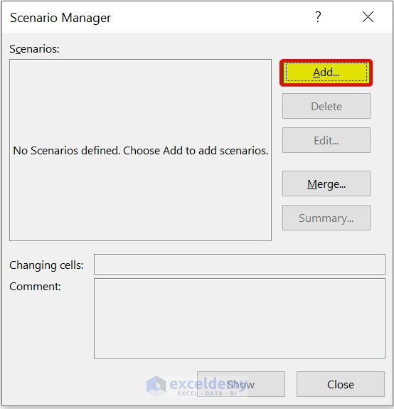
• First, go to the Data From the Forecast group, select What-If Analysis > Scenario Manager.

• Then, the Scenario Manager dialog box will appear. After that, click on Add .

• Then, in the Edit Scenario dialog box, give a Scenario name . We are giving it House 2 . After that, select Changing cells .

• Next, select the range of cells C5:C9 . We will change these inputs.

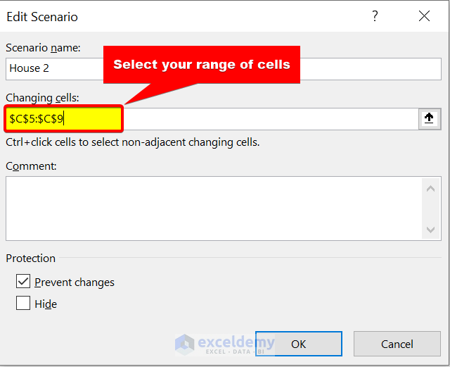
• After that click on OK .
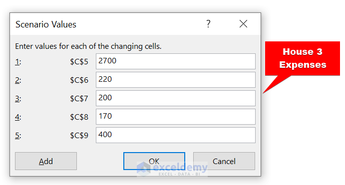
• Now, in the Scenario values dialog box, we are giving the expenses of House 2. Then, click on Ok .

• Now, we have added a scenario for House 2 . Do the same for House 3 .
• Here, we are giving these values for House 3

• We added both scenarios. Select House 2 and click on Show to see the changes.

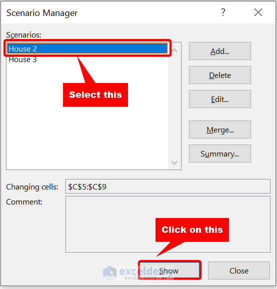
• Now, you will see these changes for House 2 .

• If you choose House 3, it will give you this total cost:

As you can see, we have successfully performed scenario analysis in Excel

Create Scenario Summary:

You can also show these effects side-by-side using the Scenario Summary.

• First, open the Scenario Manager.

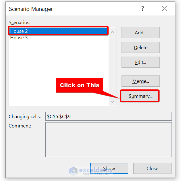
• Then, click on Summary .

• Now, select your Result cells . Here, our result cell is C10 because we were showing our Total values on that cell. Next, click on OK .

Here, you can see the side-by-side scenario summary in a different worksheet. Now, you can easily decide which House you should choose.

Read More:  How to Use Scenario Manager in Excel

Scenario Analysis in Excel: 2 Practical Examples

In the following sections, we will provide you with two practical examples of scenario analysis in Excel. We recommend you read and try all of these.  We hope it will increase your interest in scenario analysis. Hopefully, it will improve your Excel knowledge.

1. Scenario Analysis of Compound Interests in Excel

In this section, we will show you an example of the Compound interests of banks. We will create two scenarios of this example to demonstrate.

Compound interest means earning or paying interest on interest. Basically, it is one of those popular financial terms. When we think about compound interest, we consider it as gaining money. It increases our savings after a limited period.

The formula of Compound Interest:

This example will contain the same dataset. But we will calculate differently compound interests.

Suppose, you want to invest $10000 for ten years somewhere. You have got three options:

• Bank "X" is providing 5% interest compounded yearly.
• Bank "Y" is offering 5% interest compounded monthly.
• Bank "Z" is giving 5% interest compounded daily.

Now, you are in puzzlement where to apply. So, let’s use our scenario manager to find which one will provide you with more profit.

This is the dataset for Bank “X”:

We are using this formula to calculate the Estimated Balance:

Let’s create a scenario analysis.

• First, go to the Data tab. Then, from the Forecast group, select What-If Analysis > Scenario manager .
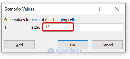
• Then, in the Edit Scenario dialog box, give a Scenario name . We are giving it Bank “Y” . After that, select cell C6 in Changing cells . Because only the number of compounding periods per year will vary here. Everything will be the same. Then, click on OK .

• Then, in the Scenario Values dialog box, enter 12. Because Bank “Y” gives 5% compound interest monthly. So, there will be 12 compounding periods per year. Next, click on OK .

• Now, we have created a scenario for Bank “Y”.

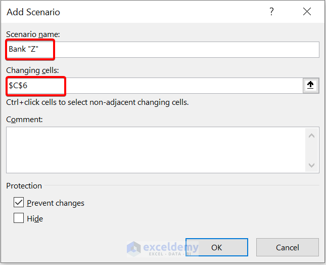
• To add a scenario for Bank “Z”, click on Add.

• Then, give this scenario the name Bank “Z”. Then, select cell C6 as the changing cell.

• Now, give the scenario values 365. Because Bank “Z” is offering 5% interest compounding daily. So, no. of compounding periods will be 365 days.

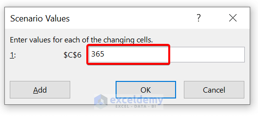
• Then, click on OK .

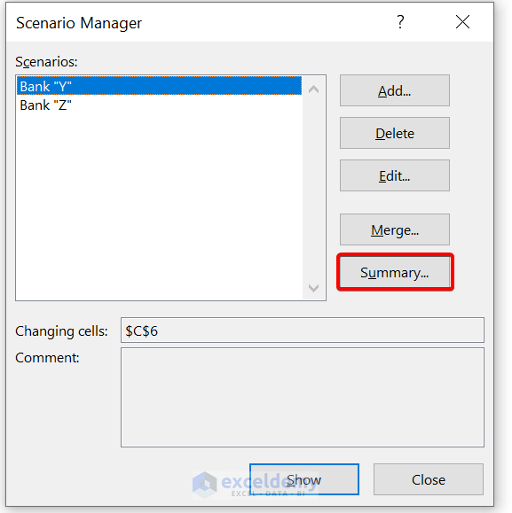
• Now, to create a scenario summary report, click on Summary . Then select cell C9 as the result cell.

• After that, click on OK .

As you can see, we have successfully created a scenario analysis in Excel. You can see the estimated balance for each compound interest of the banks.

2. Preparing Budget for an Office Tour Using Scenario Manager

In this section, we are going to show you almost a similar example as we showed earlier.

Suppose, your office has decided to go on an office tour. Now, your boss has given you the responsibility to make the budget. You have three options for choosing a place.

For this, you have made this budget:

Now, the budget you have made is for place 1. You have to make a budget for Place 2 and Place 3. After that, you have to decide which option will be better.

• First, go to Data Then, from the Forecast group, select What-If Analysis > Scenario manager.
• Then, in the Edit Scenario dialog box, give a Scenario name . We are giving it Place 2 . After that, select the range of cells C5:C9 in Changing cells . Then, click on OK .

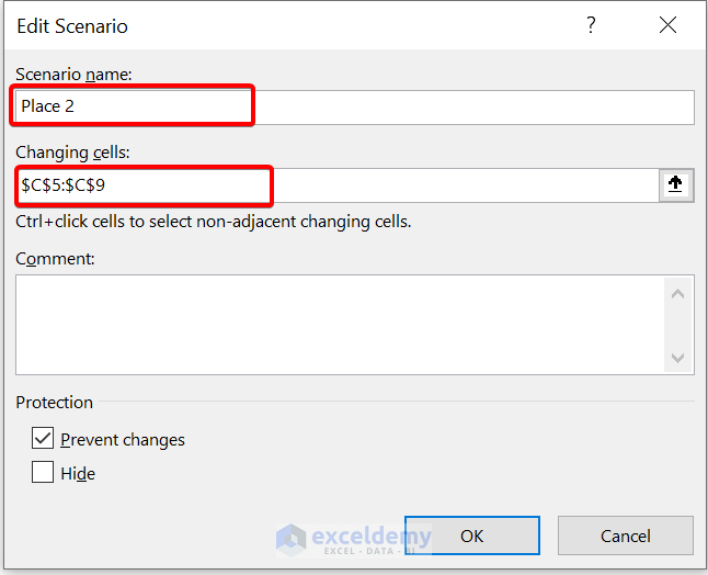
• Now, give the expenses for Place 2

• Now, we have added the Place 2 scenario. After that, click on Add to add scenario for Place 3.
• Create a Scenario for Place 3 in the same process. Now, give your expenses for Place 3.

• Now, click on OK .

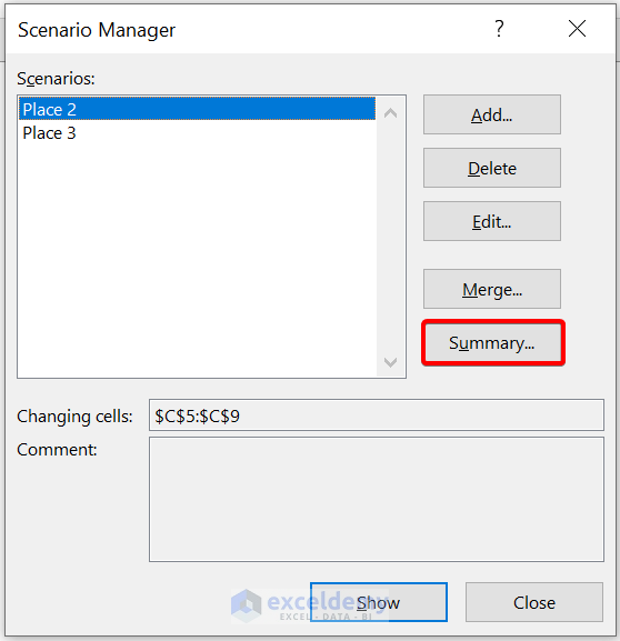
• After that, click on Summary to analyze the scenarios side-by-side. Then, select cell C10 for showing the result.

• Finally, click on OK .

As you can see, we have successfully performed the scenario analysis of an office tour in Excel.

Read More:  How to Create a Scenario Summary Report in Excel

💬 Things to Remember

✎ By default, the summary report uses cell references to recognize the Changing cells and the Result cells. If you make named ranges for the cells before you run the summary report, the report will have the names instead of cell references.

✎ Scenario reports do not automatically recalculate. If you modify the values of a scenario, those modifications will not show up in a current summary report but will show up if you build a new summary report.

✎ You don’t require result cells to generate a scenario summary report, but you need to require them for a scenario PivotTable report.

Download Practice Workbook

Download this practice workbook.

To conclude, I hope this tutorial has provided you with a piece of useful knowledge to create a scenario analysis in Excel. We recommend you learn and apply all these instructions to your dataset. Download the practice workbook and try these yourself. Also, feel free to give feedback in the comment section. Your valuable feedback keeps us motivated to create tutorials like this.

Keep learning new methods and keep growing!

Further Readings

• How to Create Scenarios in Excel
• How to Create a Scenario with Changing Cells in Excel
• How to Edit Scenarios in Excel
• How to Remove Scenario Manager in Excel

<< Go Back to Excel What-If Analysis Scenario Manager | What-If Analysis in Excel  |  Learn Excel

What is ExcelDemy?

Tags: Excel What If Analysis Scenario Manager

A.N.M. Mohaimen Shanto, a B.Sc. in Computer Science and Engineering from Daffodil International University, boasts two years of experience as a Project Manager at Exceldemy. He authored 90+ articles and led teams as a Team Leader, meticulously reviewing over a thousand articles. Currently, he focuses on enhancing article quality. His passion lies in Excel VBA, Data Science, and SEO, where he enjoys simplifying complex ideas to facilitate learning and growth. His journey mirrors Exceldemy's dedication to excellence and... Read Full Bio

Thank you for sharing Shanto! I found a problem that also appears in your article. In the Scenario Summary for section 1 example, the “Current Values” column shows data for House 3 as the result of the last operation. How to retrieve the original data for House 1?

Hello HOWARD, Thanks for asking this important question. Basically scenario summary will show the latest dataset in the current values column. As we changed the scenario by clicking OK.

Now, this is not a wonderful solution. But it may help you.

1. Copy the original dataset to a new sheet. 2. Then go to Scenario Manager 3. Now click Summary. You will see the original data in Current Values. Thank You.

Leave a reply Cancel reply

ExcelDemy is a place where you can learn Excel, and get solutions to your Excel & Excel VBA-related problems, Data Analysis with Excel, etc. We provide tips, how to guide, provide online training, and also provide Excel solutions to your business problems.

Contact  |  Privacy Policy  |  TOS

• User Reviews
• List of Services
• Service Pricing

• Create Basic Excel Pivot Tables
• Excel Formulas and Functions
• Excel Charts and SmartArt Graphics
• Advanced Excel Training
• Data Analysis Excel for Beginners

Advanced Excel Exercises with Solutions PDF

• Contact AIChE
• Communities
• Learning & Careers
• Publications
• Careers at AIChE
• Equity, Diversity, Inclusion
• Young Professionals
• Operating councils
• Local Sections

Other Sites & Tools

Technical groups, follow aiche.

Search form

Excel Tip #5: Take Advantage of Data Tables for Case Studies

• Feb 28, 2017
• Comments (0)

Topics: 

• General Interest
• Professional Development
• General Interest (Professional Development)

Share This Post:

Share your tips, on engage.

Do you have some tips of your own about spreadsheets? If you're a member, I'd love you to share them on AIChE Engage .

Once chemical engineers develop a spreadsheet calculation, however large or small in scale, they are typically interested in running case studies. Case studies can produce results for variations in input values. Engineers very often do this manually, by copying-and-pasting calculation results into an adjacent table and then generating charts to depict the relationships. However, there is a better way.

Below, we illustrate the application of Excel’s Data Table tool for a “one-way” case study. A set of input values is mapped into an input cell, and the corresponding values from a result cell are tabulated. This feature is live on the spreadsheet and is implemented with Excel’s TABLE array function.

We can use the Data Table tool to study the cash flow table (a) below. In this example, the internal rate of return (IRR) and net present value (NPV) are calculated based on net cash flows in years 0 through 5. The underlying formulas for the first several columns are shown in (b) below; the rest follow the established pattern.

To carry out a case study of IRR versus selling price, we set up a column of candidate selling prices and a pointer formula to IRR in the adjacent column, one row up from the selling prices (see below). Then, by invoking the Data Table command from the What-If Analysis drop-down list in the Data Tools group of the Data tab of the Ribbon, and identifying the Column Input cell as the Selling Price (named Sell), we can flesh out the table.

This is a live case study, so when another parameter, such as the inflation rate, is changed, the values update automatically.

The Data Table feature also allows for two-way case studies. To construct a two-way case study, place a column of values for one input parameter on the left of the table and a row of values for a second input parameter in the top row of the table. Then, place the pointer formula, or rule, in the empty cell in the upper left-hand corner of the table.

Excel’s Data Table is a convenient, efficient tool for carrying out case studies using spreadsheets as a calculation engine. Several case studies can be adjoined to a spreadsheet calculation, anticipating questions that might arise about the sensitivity of results to changes in input parameter values. Take advantage of Data Tables!

More tips and techniques

If you're just joining us, check out the entire series . And if you want a full crash course instead of just helpful tips, you should check out the AIChE Academy's " Spreadsheet Problem-Solving for Chemical Engineers ," where these tips come from, and also check out the other Excel courses available through the AIChE Academy at www.aiche.org/academy .

Want more Excel tips for chemical engineers?

If you know you want to delve even deeper than this blog series – or if our Excel tips leave you hungry for more – be sure to check out AIChE’s  virtual combo course on spreadsheet problem solving and VBA programming . It’s taught by David E. Clough, the author of this series, and combines two of AIChE’s most popular spreadsheet courses, Spreadsheet Problem-Solving for Chemical Engineers and Excel VBA Programming for Chemical Engineers.

Do you have some tips of your own about spreadsheets? If you're a member, I'd love you to share them on AIChE Engage .

This Excel spreadsheet series is drawn from an article by David Clough that appeared in AIChE's CEP Magazine .  You can find the current issue and an extensive archives of back issues at  www.aiche.org/cep .

Advanced Excel for Business Analysis & Data Visualization

• Excel Functions
• Excel Formulas
• Excel Macro
• Training Programs

Excel Case Studies for Advanced Excel Users

[tcb-script async=”” src=”https://pagead2.googlesyndication.com/pagead/js/adsbygoogle.js”][/tcb-script][tcb-script] (adsbygoogle = window.adsbygoogle || []).push({});[/tcb-script]

​Compare 2 worksheets

​A participant came to me at the end of the course and asked if there is a easier way to compare 2 worksheets. This seems like a simple task of using VLOOKUP. Just enter the VLOOKUP formula into a column in one of the worksheet and refer to the other worksheet for comparative values.That’s what usually people need.

​But for her problem, it is not so simple. Her worksheet which contains employee data (e.g. employee number, name, reporting manager, departmet) has multiple columns and rows and all the cells need to be compared against the other worksheet. To add to the challenge, the rows are not in the same order, meaning that the employee in row 10 may not be presented in Row 10 of the other worksheet. So that is the best way to compare the 2 worksheets?…. more details on compare 2 worksheets

​Excel Calendar

​This is a wonderful creation by John Walkenbach. The solution makes extensive use of the YEAR, MONTH, DAY and WEEKDAY formula. Understanding how Excel stores dates is a pre-requisite to understand how all the 4 formulas work as one. But another main ingredient is the use of array formula. The employ of the IF formula helps to clean up the monthly calendar so that only days related to that particular month is displayed.

​The conditional formatting makes use of SUMPRODUCT, which I called a super formula. This formula can do wonders. Compared this formula with the new SUMIFs and COUNTIFs, it still wins. SUMPRODUCT allows the use of formulas within the conditions while SUMIFs and COUNTIFs do not. VLOOKUP and AND are also used in conditional formatting to generate this perfect solution. More details can be found in this excel calendar write-up .

​ Return to the top of case studies

New! Comments

Have your say about what you just read! Leave me a comment in the box below.

Share this page:

What’s this?

Enjoy this page? Please pay it forward. Here’s how…

Would you prefer to share this page with others by linking to it?

• Click on the HTML link code below.
• Copy and paste it, adding a note of your own, into your blog, a Web page, forums, a blog comment, your Facebook account, or anywhere that someone would find this page valuable.

Excel Courses for Business Professionals

How to sleep and lose weight

Copyright © advanced-excel.com 2007 – 2019. All Rights Reserved. Privacy Policy

Microsoft® and Microsoft Excel® are registered trademarks of Microsoft Corporation.

advanced-excel.com is in no way associated with Microsoft

Popular Courses

Useful Links

Links I found useful and wanted to share.

Search the website

Industry Case Studies

We have helped countless small and large organizations automate & streamline their operations saving them time and money

Expert Excel & Database Solutions

View case studies of our excel, access, sql hybrid development below:, insurance industry.

Processing insurance claims can be challenging due the vast amount of data that is required and the process is typically very manual. eSoftware Associates was hired to improve a manual claims processing system as well as a build a quoting tool for another firm.

Case Study:

Construction Industry

Efficiently managing project resources in the construction industry can be very difficult. ESW built a calculation engine that would forecast full-time and contractor resource availability as they rolled off and on to projects. A huge win for the executive team when it came to resource planning.

Whitepaper:

Automotive Manufacturing Case Study

There are a tremendous amount of moving pieces in the automotive manufacturing industry that prohibits one software solution from servicing all. ESW has provided cost savings and extreme value over the past decade by designing BOM, estimate and inventory systems per specific client requirements.

Manufacturing Engineering Industry

Attempting to create a single process for all of your products and custom manufacturing processes can be extremely burdensome since there is so many pieces of data to consider. ESW aligns manufacturing business with proper technology in order to grow without interruption.

Finance Industry

Based on the nature of the finance industry, ESW has had a vast array of opportunities to assist, streamline and develop efficient systems related to financial models, database repositories, reporting and various visualization analytics for financial companies.

Oil & Gas Industry

ESW works in many facets of the Oil & Gas industry from assisting various drillers in analyzing their findings to helping pipelines and worldwide oil transport companies make sense out of their rig or oil related data.

Legal Industry

At ESW, we partner with law firms in order to provide case intensive data analysis, interpretation and documentation for court proceedings and settlement activity. Our teams will even provide expert testimony as is necessary and today’s legal world.

Government Case Study

ESW works with local, state, federal and approved foreign government entities in a variety of capacities which include general technology consulting, supplemental data analysis, Microsoft application support & development and training. Learn how ESW streamlined an entire country in 2016.

Health & Wellness Case Study

Fast growing startups need access to accurate information and reports for management to review at the drop of a hat. ESW takes pride in wrangling the suite of Microsoft applications to provide flexible retrieval of information in a fast-paced environment.

Pharmaceutical / Healthcare Industry

Learn how ESW has developed compliant healthcare and pharmaceutical Microsoft Excel forms & database applications for various organizations over the past decade.

Education & Non-Profit Industries

ESW works with many colleges all over the country providing support for various Microsoft related applications and training to fill in gaps where in-house resources do not exist. Many of these clients have partnered with ESW for many years.

Retail Industry

ESW works with many understand all of your data in a quickly changing marketplace becomes burdensome with out-of-the-box solutions and why we have helped numerous Fortune 500 retail chains improve their data awareness and analytics.

Fill out our  contact form or call us right now at to find out more about our Insurance related services. Whether you need Excel data related Analysis or Excel / Microsoft VBA programming, we will save you time and money.

Join 307,012+ Monthly Readers

Get Free and Instant Access To The Banker Blueprint : 57 Pages Of Career Boosting Advice Already Downloaded By 115,341+ Industry Peers.

• Break Into Investment Banking
• Write A Resume or Cover Letter
• Win Investment Banking Interviews
• Ace Your Investment Banking Interviews
• Win Investment Banking Internships
• Master Financial Modeling
• Get Into Private Equity
• Get A Job At A Hedge Fund
• Recent Posts
• Articles By Category

The 3-Statement Model: Full Tutorial for a Timed 90-Minute Modeling Test

If you're new here, please click here to get my FREE 57-page investment banking recruiting guide - plus, get weekly updates so that you can break into investment banking . Thanks for visiting!

A long time ago, we received one complaint/criticism more than any other:

“All your models start from templates ! What about case studies where I have to start from a blank Excel sheet and do not get any data, formatting, or schedules?”

We did this mostly to save time : entering the historical information and setting up the formatting, layout, etc., usually takes at least 30 minutes and sometimes up to several hours.

But there is also value in learning how to build a full model from scratch .

We’ll cover a 90-minute 3-statement modeling test here and explain how to use the company’s financials, 10-K, and investor presentation to do everything.

WARNING: You must have a decent-to-high Excel proficiency to follow along and finish this in the allotted time.

The video walkthrough below has captions for some of the Excel shortcuts, but it’s not a full Excel tutorial, and we assume you already know the basics.

What is a 3-Statement Model?

In financial modeling , the “3 statements” refer to the Income Statement, Balance Sheet, and Cash Flow Statement.

Collectively, these show you a company’s revenue, expenses, cash, debt, equity, and cash flow over time, and you can use them to determine why these items have changed.

In a 3-statement model, you input the historical versions of these statements and then project them over a ~5-year period.

In real life, you do this to value companies, model transactions, and determine whether the company’s expected growth, margins, and cash flow metrics are plausible.

For example, if the company claims it will generate $5 billion of Free Cash Flow and use it to repay $1 billion of Debt and issue $4 billion in Dividends, is that realistic?

Will the company generate more or less cash flow? Might it need outside financing? How do the numbers change if market conditions worsen?

Banks like to test this topic because it’s a quick way to assess who’s proficient in Excel, accounting, and financial modeling.

If you cannot read or interpret a company’s historical financial statements, you won’t be working on complex deals anytime soon.

Types of 3-Statement Modeling Tests

Most 3-statement models and case studies fall into one of three categories:

• Blank Sheet / Strict Time Limit: These are more about working quickly, knowing the Excel shortcuts, simplifying, and making decisions under pressure.
• Template / Strict Time Limit: These tests are more about entering the correct formulas, justifying your assumptions, and answering questions based on your model’s output.
• No Strict Time Limit: These case studies are more about using outside research and data to justify your assumptions for the revenue, expenses, cash flow, etc. You might also have to give a presentation based on your findings.

The “strict time limit” could be anything from 30 minutes to 3-4 hours, and the complexity increases as the time limit increases.

The “no strict time limit” type might give you several days or even 1 week+.

There is still a deadline, but you don’t need to rush around like a madman to finish.

The 90-Minute 3-Statement Model from a Blank Sheet

For this tutorial, I picked an example where you start from a blank sheet and review the company’s filings and presentations .

So, you must demonstrate Excel proficiency and the ability to interpret data and make reasonable assumptions.

You can get the case study prompt, the company documents, and the completed Excel file below:

• 90-Minute 3-Statement Model – Case Study Prompt (PDF)
• 90-Minute 3-Statement Model – Completed Excel File (XL)
• Overview of Main Points in 90-Minute 3-Statement Modeling Test – Slides (PDF)
• Otis – 10-K (PDF)
• Otis – 10-K in Excel Format – Raw (XL)
• Otis – User-Friendly 10-K in Excel with Swapped Columns (XL)
• Otis – Investor Presentation (PDF)

There is no “blank” or “beginning” file because we create a new sheet in Excel and enter everything from scratch in this tutorial.

You can get the video version of this entire tutorial below:

Table of Contents:

• 2:35: What is a 3-Statement Modeling Test?
• 5:54: Part 1: Inputting the Historical Financial Statements
• 15:31: Balance Sheet Entry
• 24:14: Cash Flow Statement Entry
• 35:11: Part 2: Income Statement Projections
• 50:12: Part 3: Balance Sheet Projections
• 57:51: Part 4: Cash Flow Statement Projections
• 1:07:12: Part 5: Linking the Statements
• 1:10:59: Part 6: Debt and Stock Repurchases
• 1:19:16: Part 7: Model Checks, Review, and Final Comments
• 1:22:35 : Recap and Summary

This example is not taken from our courses – it’s new for this article – but it is similar to some of the case studies in our Core Financial Modeling course :

Core Financial Modeling

Learn accounting, 3-statement modeling, valuation/DCF analysis, M&A and merger models, and LBOs and leveraged buyout models with 10+ global case studies.

The full course has 3-statement models with and without templates for additional practice. If you want more advanced 3-statement models with additional schedules, the Advanced Financial Modeling course might be more appropriate since it goes into far more depth in each case study:

Advanced Financial Modeling

Learn more complex "on the job" investment banking models and complete private equity, hedge fund, and credit case studies to win buy-side job offers.

3-Statement Model, Part 1: Inputting the Historical Statements

You could attempt to input the data by copying and pasting from the PDFs, but it’s far more efficient to link directly to the Excel or CSV files.

A few tips:

• Swap the Excel columns, so they go from oldest to newest (see below).

• On the Income Statement , use positives for revenue and other income sources and negatives for all expenses and outflows, as it will be easier to check your work that way.

• Consolidate smaller line items as much as possible; you ideally want ~5 items on each side of the Balance Sheet (maybe 10 at the most) and only a few items in each section of the Cash Flow Statement.

As you proceed, you can check your work by summing up the sections and comparing the totals to the company’s numbers.

3-Statement Model, Part 2: Income Statement Projections

The case study document says that we need to use “something more complicated” than a simple percentage growth rate for Revenue:

But the investor presentation and 10-K do not make it easy to find unit-by-unit data.

We’d ideally like to project new escalators and elevators sold, forecast the average prices, and assume a certain percentage of these new units go into “Service Units,” generating Services revenue in future periods.

It would also be helpful to know about something like the degree of operating leverage , so we could better forecast different expenses.

But we can’t find enough solid data to do this within the strict time limit, so we simplify and use Market Share and Market Size to project the New Equipment Revenue, with the Services Revenue based on the company’s estimates for the growth in Service Units:

The Cost of Products, Cost of Services, and Operating Expenses are simple percentages of Revenue, and the Taxes and NCI Net Income are based on average historical percentages:

3-Statement Model, Part 3: Balance Sheet Projections

In this part, we focus on projecting the Working Capital line items , such as Accounts Receivable (AR), Inventory, and Accounts Payable.

With more time/information, we might also use metrics like the Days Sales Outstanding or Cash Conversion Cycle to forecast some of these items.

The key point is that the absolute numbers do not matter .

What matter is the Change in Working Capital on the Cash Flow Statement since that affects the company’s cash flow and ability to repay Debt and repurchase Stock.

If the Change in WC has been positive as the company has grown, it should stay positive and in the same range in the future (and vice versa if it has been negative or near-0).

We make most of these items simple percentages of Income Statement lines such as Revenue, COGS , or Total Expenses:

Once we do this and set up the projections, we can calculate the Change in Working Capital on the Cash Flow Statement to check our work:

We also simplify the Operating Leases here by making the Operating Lease Assets a percentage of Operating Expenses and assuming the Operating Lease Liabilities change by the same amount each year.

Lease accounting is more complicated in real life and under IFRS, but this approach is fine for a U.S.-based company.

3-Statement Model, Part 4: Cash Flow Statement Projections

Most of the key line items here, such as CapEx and Depreciation & Amortization, are simple percentages of Revenue:

A few line items, such as the ones for Pension Contributions and Noncontrolling Interests , are more complex to project “correctly,” but we don’t have time to do so here.

One exception to these simple rules is the Dividends line, which we forecast based on the Dividend Payout Ratio (i.e., Dividends / Net Income) (for more, see our tutorial on the dividend yield ).

In this case, the company provides specific guidance on the Dividend Payout Ratio, so we increase it slightly over the period to match their targets (see below).

The bolt-on acquisitions are also a bit different because the company estimates $50 – $100 million per year in acquisition spending in its investor presentation , so we pick the middle of the range and assume $75 million each year:

Strangely, CapEx is below D&A in each projected year, but it’s not necessarily “wrong” for a low-growth company like this one.

We would examine this point and refine these projections if we had several hours or days to complete this case study.

3-Statement Model, Part 5: Linking the Statements

We already have the Working Capital items and the Operating Lease Assets and Liabilities linked on the Balance Sheet, so there are only a few items left to complete.

The main rules are:

• Assets Side – When linking an Asset to a line on the CFS, you start with the old Asset on the Balance Sheet and subtract the matching line on the CFS. This is because cash outflows represent increases in Assets, and cash inflows represent decreases in Assets .
• Liabilities & Equity Side – It’s the opposite: add the line items on the CFS to the old numbers on the Balance Sheet.

Here’s what we do for the remaining line items:

• Cash: Old Cash Balance + Net Change in Cash on the CFS.
• PP&E/Goodwill/Intangibles: This simplified/consolidated line item equals the old balance minus CapEx minus D&A. Due to the signs on the CFS, CapEx increases this number, and D&A decreases it.
• Other Assets: Start with the old number and subtract Acquisitions and the “Pensions/Other” line.
• Total Debt: Old Debt Balance + Change in Debt from the CFS.
• Noncontrolling Interests (NCI) : Old NCI Balance + NCI Net Income from the CFS + NCI Dividends from the CFS.
• Common Shareholders’ Equity (CSE): Old CSE + Net Income + Dividends + Stock Repurchases + Other Items + FX Rate Effects.

This last one is a “catch-all” for everything else on the CFS that has not yet been reflected on the Balance Sheet, and it’s sometimes also known as the Statement of Owner’s Equity .

Our Balance Sheet balances after completing these links, which is a good sign:

But we’re not done because the Change in Debt, Stock Repurchases, and Interest Expense lines are still blank.

3-Statement Model, Part 6: Debt and Stock Repurchases

The case study document tells us to “follow company guidance” for these last few line items.

On slide 41 of their investor presentation , Otis provides an estimated percentage split of its Free Cash Flows over the next 3 years:

We already have the Dividends and Acquisitions, so we’ll use a simple logical check for the Debt and Stock Repurchases based on the $3 billion Minimum Cash from the case document :

• Step 1: Does the company have Excess Cash Flow in this period? In other words, is its Beginning Cash + Net Change in Cash – Minimum Cash a positive number? If so, it can use that cash flow to repay Debt principal and repurchase Stock.
• Step 2: Based on the chart above, we assume an 85% / 15% split between Stock Repurchases and Debt Principal Repayments.
• Step 3: If the company has a Cash Flow Deficit , i.e., Beginning Cash + Net Change in Cash – Minimum Cash is negative, it must issue additional Debt to fund its operations.

You can see the logic below:

With these formulas, we can now add these links to the Cash Flow Statement and set the “Other” line item in Cash Flow from Financing to ~2% of Debt Issuances to represent the issuance fees.

The last line item is the Interest Expense on the Income Statement.

We can calculate the average interest rate on Debt in the previous years, but we don’t know how it will change in the future.

Interest rates were rising at the time of this case study, but if the company’s Debt has fixed rates and matures far into the future, it may not matter.

We can search for “long-term debt” in the 10-K and get a quick answer:

Since most of this company’s Debt matures after the 5-year projection period, the average rate probably won’t increase by that much in this period.

But there are ~$3.4 billion of maturities in the next 5 years, so we increase the average interest rate from 2.0% to 3.5% and use these numbers to calculate the Interest Expense:

To avoid circular references, we can use the Beginning Debt balance to calculate the interest expense as well (for more, see our tutorial on how to find circular reference in Excel ).

3-Statement Model, Part 7: Model Checks, Reviews, and Final Comments

At a high level, this model confirms that most of the company’s claims are reasonable.

For example, Otis generates just over $5 billion in FCF over the next 3 years, and it spends the expected amounts on Dividends, Acquisitions, and Stock Repurchases:

Its Free Cash Flow Conversion, which the company defines as FCF / Net Income, also stays well above 100%.

We’ve completed the model and met the requirements within the 90-minute time limit, so this attempt was successful.

However, there are some issues that we would fix with more time and resources:

• Formatting – It’s not pretty right now. We must clean up the number formats, add input boxes for the projections, fix the color coding, add headers/footers, etc.
• Revenue, Expense, and Cash Flow Detail – It’s better to project Revenue based on individual units sold and link the Product and Service segments to each other, such that New Units Sold drives Service Revenue in future periods; items like Operating Expenses should be linked to the Employee Count, and CapEx should be linked to the company’s production capacity.
• Scenarios – Finally, we always evaluate companies across multiple scenarios in real life. What happens if the market growth changes? What if the company’s market share falls? What if its expenses rise? This model is not robust enough to support these scenarios or sensitivities.

How to Master the 3-Statement Model

This example is more difficult than the average 3-statement modeling test.

If you don’t have moderate-to-high Excel proficiency, you could easily spend an entire day (or more) on this.

But if you can finish in 2-3 hours, you’re at the level where you can improve your times with repeated practice and eventually do this in 90 minutes or less.

You don’t need to score 100% to “pass” these tests; the median scores tend to be very low.

Your goal should be to finish the model , and if you can’t complete everything, simplify so that you can answer at least the main questions by the end.

If you have an upcoming 3-statement modeling test, get as many examples as possible and complete them.

If you can’t find good examples, pick companies you follow, download their statements and investor presentations, and do what we did here: start from scratch and give yourself a few hours to build a simple 3-statement model.

If you improve over time and find it interesting to pick apart companies and business models, great.

If not… well, maybe the finance industry is not for you.

Further Learning

You might be also interested in this tutorial on balance sheet forecasting .

About the Author

Brian DeChesare is the Founder of Mergers & Inquisitions and Breaking Into Wall Street . In his spare time, he enjoys lifting weights, running, traveling, obsessively watching TV shows, and defeating Sauron.

Free Exclusive Report: 57-page guide with the action plan you need to break into investment banking - how to tell your story, network, craft a winning resume, and dominate your interviews

Learn Valuation and Financial Modeling

Get a crash course on accounting, 3-statement modeling, valuation, and M&A and LBO modeling with 10+ global case studies.

Excel Tutorial

Excel formatting, excel data analysis, table pivot, excel functions, excel how to, guided projects, excel examples, excel references.

Excel is the world's most used spreadsheet program

Excel is a powerful tool to use for mathematical functions

Start learning Excel now »

Learn Excel

Examples in Each Chapter

We use practical examples to give the user a better understanding of the concepts.

Copy Values Tool

Example values can be copied from the tutorial and into your spreadsheet, making it easy for you to tag along step-by-step:

Advertisement

Case Based Learning

We have created active learning activities, so you can test and build your knowledge. Making the learning experience more fun and engaging.

Solve Case »

Why Study Excel?

Excel is the world's most used spreadsheet program.

Example use areas:

• Data analytics
• Project management
• Finance and accounting

Test Yourself With Exercises

Excel exercise:.

Complete the Excel formula:

Start the Exercise

My Learning

Track your progress with the free "My Learning" program here at W3Schools.

Log in to your account, and start earning points!

This is an optional feature. You can study at W3Schools without using My Learning.

COLOR PICKER

Contact Sales

If you want to use W3Schools services as an educational institution, team or enterprise, send us an e-mail: [email protected]

Report Error

If you want to report an error, or if you want to make a suggestion, send us an e-mail: [email protected]

Top Tutorials

Top references, top examples, get certified.

• Real Estate

Home » Business » Free Case Study Templates & Examples (Word, PDF)

Free Case Study Templates & Examples (Word, PDF)

A case study template is used to make a report of an event, problem, or activity in an effective way. With the help of this template, you don’t have to think that what to include in your report. However, you just have to focus on a person, group, or event you are studying.

Table of Contents

What is a case study?

Generally, a case study is a kind of research methodology and usually used in social sciences. If people do a case study then they have to study an issue from a real-life perspective. Moreover, such type of studies demands in detail analysis of a person, a group, or an event. You may also like Remote Work Policy Template .

Different Types of Case Study Templates?

There are different types of templates that you can use for your case study;

• Student case study template
• Nursing case study template
• Clinical case study template
• Basic psychology case study template
• Treatment injury case study template

In addition, you can also create these templates on your own or you can download them from any website. There are no specific formats for these templates. You have to create or download those templates that suit your own needs.

What are the benefits of using a case study in business?

Using case study in the business provides you several benefits such as;

• A case study assists you to influence customers more efficiently. It makes you able to raise awareness on how to fulfill the requirements of customers more efficiently.
• Next, the information in the report will help you to encourage empathy in its readers. If you use the real-life issues and then explain how your product solves those issues will encourage the customers to use your product.
• Moreover, when you discuss the customers’ issues and questions in your case study it shows that you care and understand the customers.
• With the help of this report, you can strengthen your brand. Hence, it depends on real-life situations, it becomes relatable. You can also develop an emotional relationship with your customers. Furthermore, this report shows that you have everything that customers need.
• Above all, you can use this report to create other written works for your business. You should also check Employee Clearance Form Template .

Basic Psychology Phase One Case Study Template

Blog and Case Study Template

Clinical Case Study Template

Community Engagement Case Study Template

Firebird SQL Case Study Template

Grow’s Case Study Template

IBM Case Study Template

JISC Case Study Template

Memorial Hospital Case Study Template

Nursing Case Study Template

School Education Case Study Template

Social Values and Health Priority Setting Case Study Template

Student Case Study Example Template

Ultimate Case Study Template

How to write a case study?

Here are some guidelines that you bear in mind during or before writing a case study;

At first, you should identify what type of case study you are going to perform. You should strategize your case study well.

Next, in business, you have to pay attention to customers. If you are going to sell products or services, then think about your customers and their needs.

Most importantly, gather extensive knowledge about your project before making a case study. Without enough knowledge, you won’t be able to create an effective document. You may also see Employee Handbook Template .

If you want to present, the best side of your business then finds those customers who have the best experience with your product or services. Then, include their testimonials in your report.

In conclusion, case study templates make you able to create a study that surely makes your business stand out.

You May also Like

Sharing is caring!

• Excel World Championship Sample Case #1: Knowledge Is Power /

Excel World Championship Sample Case #1: Knowledge Is Power

Anybody who’s anybody has heard of the hot new sport sweeping the world: competitive Excel ! Every year, dozens of the best analysts, accountants, and mathematicians face off to see who can best model extremely complicated problems within thirty minutes. The “sport” first gained widespread attention during the Covid-19 lockdowns and has been growing in popularity ever since; next week’s championship will take place in HyperX Arena in Las Vegas and be televised in bars on the other side of the country .

If this is the first time you’re hearing about all this, take a moment to check out People Make Games’s short documentary on the topic:

Personally, I don’t think my prowess at Excel quite reaches the levels of storied champions like Diarmuid Early or Laurence Lau (yet…). However, it came to my attention that the website for the Financial Modeling World Cup offers free sample cases adapted from actual tournament matches from previous years. With just a few minor tweaks, these would work perfectly as projects for my data analytics portfolio.

In this and future installments, I will use these sample cases as a jumping off point. Since I’m not doing these in a competitive context, I’m dispensing with the thirty-minute time limit and the graded questionaire. Instead, I will take the results and visualize them for the sake of the imagined stakeholders. Along the way, I will describe my process and the challenges I faced.

Scenario: Knowledge is Power #

This sample case (entitled “Knowledge Is Power” on the download page ) tasks us with modeling future revenue for an online education company named Oxbridge Inc, which currently operates in the United States and Australia. They’ve become very successful during the pandemic, and they’re now planning to pitch to potential investors to fund their expansion.

Provided with the pricing and membership for five different programs (Dot, Line, Triangle, Square, and Star) along with projected monthly rates of membership growth and inflation, we have to model the next five years of monthly revenue starting in January 2022. This would be relatively simple if it weren’t for the following complications:

• All numbers must be reported in US dollars, so Australian revenue needs to be converted after applying its own specific inflation rate.
• Membership prices for each class need to keep pace with inflation and must rise in $5 increments.
• Prices can’t change too quickly. Oxbridge has recently instituted a policy of not changing any prices until at least three classes in the same country are closer to the next $5-increment than the current price. For example, a membership that currently costs $24.99 won’t jump to $29.99 until it’s actual inflation-adjust price is at least $27.49 and there are at least two other membership types that also qualify.

These are the assumptions on which our analysis will rely.

This case looks like it will require conditionals based on other conditions, so we have our work cut out for us. Let’s first start with the number for the USA.

First, we’ll need to plot out all the dates and their corresponding inflation rates. Each inflation rate is assumed to hold for the entire year, so we need to make sure that the rate switches over every January. From there, it’s simply a matter of adding the monthly interest for each class:

The Prices for the USA classes.

So how do we trigger the actual price increases below? This is where the SUMPRODUCT function comes in. With this formula, we can count the number of times where values in the range surpass the halfway threshold for the next $5-increment:

Using the SUMPRODUCT function to compare the inflation-adjusted price with the previous month’s prices.

Now it’s the moment of truth: we need a conditional function predicated on both the difference in prices and the number of classes that month to meet that threshold. Obviously we’re going to us the IF function, but more importantly, we’ll need to use the AND operator to fit both conditions:

Using the IF and AND functions to change prices in $5-increments.

As a side note, I found it interesting that Excel’s AND is a function, as opposed to a mere operator like in Python or R. This makes it slightly weird to read since AND doesn’t come between the two conditions.

We can then work on membership numbers and their monthly growth rate. We set up the months and growth rate much in the same way as we did for the prices above, then plug in the starting numbers and iterate the monthly formula for each class:

Projecting future membership of each class using the expected monthly growth rate.

Now it’s just a matter of multiplying each class’s monthly cost by its monthly users:

Projecting revenue by using each class’s membership and monthly cost.

Australia #

The sheet for the Australian branch follows a similar pattern as the sheet for the USA:

Determining the interest-adjusted prices for each Australian class.

The major difference is that all prices are in Australian dollars, so I need to convert these into US currency using the provided conversion rates:

Converting Australian dollars to US dollars.

Just like the inflation rate, the conversion rate is assumed to remain the same for each year. We need to double check that the number changes beginning with each January.

Visualization and Analysis #

Now it’s time to import the resulting revenue into the next sheet and add the revenue for both branches together:

We can use Excel’s charts to prepare a presentation for potential stockholders. These line charts describe the projected overall revenue as well as the revenue for each branch:

Monthly revenue for the US branch.

I’ve elected to include revenue for each class since it might help stakeholders strategize and make informed marketing decsions. Pie charts are often discouraged these days because they can sometimes be poorly designed, but in this case, I thought one might be helpful in visualizing how much each type of class contributes to revenue:

I’d say these projections are very reliable in the first couple years, but caution making any decisions based on the fourth and fifth years. We’re working with starting assumptions here, not data, so the numbers become less credible the further we move away from the starting state. For example, starting in 2024, the prices rise every month in at least four classes, ultimately defeating the intent of the company’s policy not to raise prices too frequently. It also beggars belief that the US branch will more than double it’s revenue to $225 million dollars starting in September 2025. If this were a real-life business situation, I would try to find a public or internal dataset to temper these projections or at the very least double-check the starting assumptions provided.

Conclusion #

This was a fun exercise and I’m looking forward to the next one. Some final thoughts on the process:

• At a certain point, I wondered if it would have been better to have chosen a long format over the wide format (i.e. long columns vs. long rows). In the next project, I’ll try to work with both simultaneously so I don’t paint myself into a corner.
• Excel is a powerful application, but Google Sheets rates higher in my book in terms of its usability. For example, I’ve never had problem making pivot tables in the latter, but for some reason, Excel is super fussy about it and won’t even let you begin one until every single thing is in the exact right place.
• I surprised myself with how much I missed creating charts using Python libraries like matplotlib and Seaborn. Sure, the process can be tedious at times, but at least every single element is theoretically customizable. Excel’s charts have a large array of options, but they’re split across several menus and sub-menus and sub-menus of sub-menus. If I can’t find the option I’m looking for, I can never be sure if it’s because it simply doesn’t exist or I haven’t plunged into the menus deeply enough. In short, the general release of Python for Excel can’t come soon enough!

If you’d like to download my Excel workbook and double check my work, click here ! Feel free to message me on LinkedIn if you have any questions or suggestions.

JOIN SOMEKA BUSINESS: Subscribe to Business Membership for exclusive benefits! Dismiss

How to use Excel Solver for Linear Programming: Solving Optimization Problems

• Updated on December 20, 2023

basToday we’re going to explain an advanced feature of Microsoft Excel. Here’s a comprehensive guide on Excel Solver Linear Programming to solve optimization problems. Solver will help you solve linear and non-linear problems.

Let’s begin!

Table Of Content

1. What’s Excel Solver? 2. How to add Solver to Excel? 3. How to add Solver to Excel on my Mac? 4. Where’s Solver in Excel? 5. How to use Excel Solver for Optimization Problems? 6. What is Optimization and Linear Programming? 7. Real-Life Example 8. Final Words

1. What’s Excel Solver?

Excel Solver is a tool that you can add to Microsoft Excel. When you need to find the best answer for a problem with certain constraints, this is a powerful tool you can use.

It basically lets you make the most or least of a certain number (usually cost or profit) within a set of variables and limits . A lot of people in areas like finance, operations management, and engineering use Solver to do sensitivity analysis, linear programming , and nonlinear problem solving .

2. How to add Solver to Excel?

Firstly, let’s start with adding Solver to Excel. Solver is an add-in, so you probably do not see Solver tab on your main menu by default . If so please firstly add this useful optimization tool to your Excel workbook.

To add the Solver add-in to Excel:

#Step1: Open the Options dialog box

To get to the options menu, go t o File > Options

#Step2: Manage Add-ins

On the Excel Options dialog box, go to Add-ins > Manage Excel Add-ins and click Go.

#Step3: Add the Solver Add-in to your Excel Workbook

Check the Solver Add-in box in the Add-Ins available box, and then hit OK.

It will be installed by Excel and can be found in the “Data” tab, under the “Analysis” group.

Now you have this fantastic optimization tool on your workbook.

3. How to add Solver to Excel on my Mac?

If you’re a Mac user, the installation of Solver may be a little bit different than Windows layout.

To add Solver to Mac Excel:

• Open the Excel app on your MacBook
• In Excel, go to the “Tools” menu.
• Click on “Add-ins for Excel.”
• Check the box next to “Solver” in the list of Add-ins that you can use.

When you click “OK,” Excel will turn on the Solver add-in. Solver is now on the “Data” tab.

4. Where’s Solver in Excel?

Solver is in Excel’s “Data” ta b, which is part of the “Analysis” group. Once you’ve added Solver to Excel, click on “Solver” in the “Data” tab to get to it.

Make sure it’s turned on in the Excel Add-ins if you can’t see it.

Now you have set up your Excel Solver and know where it is. Let’s see how to use it!

5. How to use Excel Solver for Optimization Problems in Linear Programming?

So, before diving into a case study, we want to give a general idea about how to use Solver in Excel.

So first let’s meet the Solver concepts.

What are Solver Parameters in Excel?

In Excel, the Solver Parameters are:

• Set Objective: Pick the cell you want to improve.
• To: Pick whether to set the goal cell to a certain value, maximize, or minimize.
• By Changing Variable Cells: These are the cells that the solver will change to reach the goal.
• Subject to the Constraints: These are the rules or restrictions that the answer has to follow.
• Choose a Way to Solve: You can pick Simplex LP for linear problems, GRG Nonlinear for nonlinear problems, or Evolutionary for problems whose answers aren’t clear or are close.

So while building your model, you should at least define your Objective, Variable Cells and Constraints.

Let’s build a very simple model now to see how the Solver works.

#Step1: Define your problem

Be sure that you clarify your objective, variables and constraints. Now let’s start Excel Solver Linear Programming simple case study.

Example Problem: We have two different products, with different units costs and unit prices. We have a total production capacity of 2.000 units. We want to find optimum production levels for each product to reach a net revenue of $6.000.

#Step2: Open your Solver window

Now we’ll first open our Solver window.

#Step3: Enter your objectives and variables

We’ll set objective and variables.

In this example our objective cell is the Net Revenue calculation cell. Then we’ll say that our objective cell should be $6.000.

And lastly, you’ll select the variable cells. In our example we select production levels for each product as variables.

#Step4: Add your constraints

We’ll now add our constraints using the parameters on Add Constraint window.

In our example, our only constraint is the production capacity. Our cell reference should not be more than 2.000 here.

#Step5: Choose your solving method

The Excel Solver gives you three different options to solve your problem.

We’ll not get into mathematical details here but they’re basically used for:

• Generalized Reduced Gradient (GRG): For problems that are smooth nonlinear.
• LP Simplex: For problems that are linear.
• Evolutionary: For problems that are non-smooth.

That’s all!

Now Solver has solved this problem and give us the optimum production levels:

Now you can keep your Solver solution or Restore original values and return to Solver dialog box.

6. What is Optimization and Linear Programming?

A mathematical method called linear programming is used to find the best solution in a model where the links between the parts are linear.

It is the process of finding the best solution for a linear problem that is limited by a set of linear limits. In this case, optimization means either making the goal function bigger or smaller, like making the most money or cutting costs as much as possible.

7. Real-Life Example to solve optimization problem with Excel Solver

Now we’ll give you an real-life example to solve more complex problems. This is a more complex problem than a basic Excel Solver Linear Programming examples.

In this case study, one of our clients requested us to prepare a simulation in Excel in order to test their algorithm before investing in a more expensive software solution.

Let’s come back to our case study.

Case: We have a matching application, which matches people (women to men) according to their hobbies.

Problem: We have 50 women and 50 men in our portfolio and we know their values and hobbies. We want to make optimum matches in order to catch maximum happiness for all users.

Below is the visual presentation of our source data and result matching table. We’ll try to make this table with maximum happiness.

What’s critique on optimization modelling?

It’s easy to find a match for a single user with the maximum common points. But this will not guarantee the maximum happiness for all our user database.

So if we couple the highest matching score people to each other, then there might be left very noncompliant couple prospects left!

That’s to say, if a couple has 9 matches but the other couple has only 3 matches, that’s the ideal solution. We’ll prefer both couples taking at least 7 as a matching score.

Then we have two constraints:

• We should maximize the average matching score across the group
• We should have a minimum matching score of X

So what we have done?

We have first created a matching matrix, in which we can see the matching scores of all possible couples dynamically.

Then we have input a calculation area on the left side with very simple mathematical calculations:

In order not to repeat this task each time, we also add a VBA code to automatize this process:

Now, we’ll try to go over the optimum levels for the two constraints explained above:

In Summary:

This tool basically:

• Puts all users in the matrix
• Calculates the matching scores dynamically.
• Runs Solver to test the optimization for the best solution in the thousands of combinations
• Then finds the most suitable solution for us and writes them to the final table.

Here’s the matching table view:

Our client here had very high-level developer team, and they made simulations based-on our model and tried to find the best algorithm for their application.

Isn’t Excel so impressive?

If you want to boost your Excel skills on functions, you should try our interactive Excel Formulas Trainer tool to practice your knowledge and speed on functions:

– This is the main menu of Someka’s Excel Formulas Trainer Tool with 30 exercises in three levels –

8. Final Words for Excel Solver Linear Programming

As a conclusion, the Solver function in Microsoft Excel is a very flexible and strong device that can handle a lot of different optimization issues.

Being built into Excel makes Solver not only powerful but also easy to use for people who are already familiar with the Excel environment. This article gives a step-by-step guide on how to use Solver’s features, from setting up the problem to figuring out what the results mean.

So hope this Excel Solver Linear programming article with how-to steps and case studies will help you to design optimization models for your linear and nonlinear problems.

Recommended Readings:

Career Guide: Data Analyst

How to Randomize a List in Excel?: A Comprehensive Guide

10 Must Know Excel Tricks that Experts use Everyday!

Related Posts

Cyclistic Case Study Using Spreadsheets, SQL and Tableau

In this case study, I analyze historical data from a Chicago based bike-share company in order to identify trends in how their customers use bikes differently. The main tools I use are spreadsheets, SQL and Tableau. Here are the highlights:

Tableau Dashboard: Cyclistic Bikeshare in Chicago

Slides: Where Rubber Meets Road in Converting Casual Riders to Cyclistic Members

GitHub: Cyclistic Case Study Repository

A more in-depth breakdown of the case study scenario is included below, followed by my full report.

Cyclistic is a bike-share company based in Chicago with two types of customers. Customers who purchase single-ride or full-day passes are known as casual riders , while those who purchase annual memberships are known as members . Cyclistic’s financial analysts have concluded that annual members are much more profitable than casual riders. The director of marketing believes the company’s future success depends on maximizing the number of annual memberships.

The marketing analytics team wants to understand how casual riders and annual members use Cyclistic bikes differently. From these insights, the team will design a new marketing strategy to convert casual riders into annual members. The primary stakeholders for this project include Cyclistic’s director of marketing and the Cyclistic executive team. The Cyclistic marketing analytics team are secondary stakeholders.

Defining the problem

The main problem for the director of marketing and marketing analytics team is this: Design marketing strategies aimed at converting Cyclistic’s casual riders into annual members. There are three questions that will guide this future marketing program. For my scope on this project, I will anlyze the first question:

1) How do annual members and casual riders use Cyclistic bikes differently? 2) Why would casual riders buy Cyclistic annual memberships? 3) How can Cyclistic use digital media to influence casual riders to become members?

By looking at the data, we will be able to first get a broad sense of certain patterns that are occurring in the two different groups. Understanding the differences will provide more accurate customer profiles for each group. These insights will help the marketing analytics team design high quality targeted marketing for converting casual riders into members. For the Cyclistic executive team, these insights will help Cyclistic maximize the number of annual members and will fuel future growth for the company.

Business task

Analyze historical bike trip data to identify trends in how annual members and casual riders use Cyclistic bikes differently. #

Data sources

We’ll be using Cyclistic’s historical bike trip data from the last 12 months, which is publicly available here . The data is made available by Motivate International Inc. under this license . The data is stored in spreadsheets. There are 12 .CSV files total:

It is structured data, organized in rows (records) and columns (fields). Each record represents one trip, and each trip has a unique field that identifies it: ride_id . Each trip is anonymized and includes the following fields:

Bike station data that is made publicly available by the city of Chicago will also be used. It can be downloaded here . In terms of bias and credibility, both data sources we are using ROCCC:

Reliable and original: this is public data that contains accurate, complete and unbiased info on Cyclistic’s historical bike trips. It can be used to explore how different customer types are using Cyclistic bikes.

Comprehensive and current: these sources contain all the data needed to understand the different ways members and casual riders use Cyclistic bikes. The data is from the past 12 months. It is current and relevant to the task at hand. This is important because the usefulness of data decreases as time passes.

Cited: these sources are publicly available data provided by Cyclistic and the City of Chicago. Governmental agency data and vetted public data are typically good sources of data.

Data cleaning and manipulation

Microsoft excel: initial data cleaning and manipulation.

Our next step is making sure the data is stored appropriately and prepared for analysis. After downloading all 12 zip files and unzipping them, I housed the files in a temporary folder on my desktop. I also created subfolders for the .CSV files and the .XLS files so that I have a copy of the original data. Then, I launched Excel, opened each file, and chose to Save As an Excel Workbook file. For each .XLS file, I did the following:

• Formatted as custom DATETIME
• Format > Cells > Custom > yyyy-mm-dd h:mm:ss
• Calculated the length of each ride by subtracting the column started_at from the column ended_at (example: =D2-C2 )
• Formatted as TIME
• Format > Cells > Time > HH:MM:SS (37:30:55)
• Calculated the date of each ride started using the DATE command (example: =DATE(YEAR(C2),MONTH(C2),DAY(C2)) )
• Format > Cells > Date > YYYY-MM-DD
• Entered the month of each ride and formatted as number (example: January: =1 )
• Format > Cells > Number
• Entered the year of each ride and formatted as general
• Format > Cells > General > YYYY
• Calculated the start time of each ride using the started_at column
• Calculated the end time of each ride using the ended_at column
• Calculated the day of the week that each ride started using the WEEKDAY command (example: =WEEKDAY(C2,1) )
• Formatted as a NUMBER with no decimals
• Format > Cells > Number (no decimals) > 1,2,3,4,5,6,7
• Note: 1 = Sunday and 7 = Saturday

After making these updates, I saved each .XLS file as a new .CSV file.

BigQuery: further data cleaning and manipulation via SQL

Since these datasets are so large, it makes sense to move our analysis to a tool that is better suited for handling large datasets. I chose to use SQL via BigQuery .

In order to continue processing the data in BigQuery, I created a bucket in Google Cloud Storage to upload all 12 files. I then created a project in BigQuery and uploaded these files as datasets. I’ve provided my initial cleaning and transformation SQL queries here for reference: initial_setup_query.sql

The results from the COUNT DISTINCT query for each table are very interesting. We can see that the three summer months have the highest trip counts, followed by alternating spring and fall months before ending with winter months:

Create quarterly tables

In order to perform analysis by season, let’s combine these tables. We’ll create Q1, Q2, Q3 and Q4 tables for analysis. We’ll have two Q1 tables– one for 20221 and one for 2022 – since we have FEB/MAR data from 2021 and JAN data from 2022:

• Table 1) 2021_Q1 -> FEB(02), MAR(03)
• Table 2) 2021_Q2 -> APR(04), MAY(05), JUN(06)
• Table 3) 2021_Q3 -> JUL(07), AUG(08), SEP(09)
• Table 4) 2021_Q4 -> OCT(10), NOV(11), DEC(12)
• Table 5) 2022_Q1 -> JAN(01)

We’ll first create 2021_Q2 and then repeat for the remaining four tables:

Clean and transform day of week

Some additional data cleaning is needed on the new table. First, we’ll update the format for day_of_week from FLOAT to STRING . Then, we’ll change the values from numbers to their corresponding day names (i.e. 1 = Sunday, 7 = Saturday. We’ll start with 2021_Q1 and repeat for the remaining four tables:

Delete old tables

Now that we have our tables organized into quarters, we can delete the original monthly tables from BigQuery. We no longer need the monthly tables since the data is available in the quarter tables. Also, it costs money to store these datasets in BigQuery.

Analysis #1: Exploratory

2021_q1 - quarterly data exploration.

We’ll select a few columns from 2021_Q1 to preview in a temporary table. This will help give us an idea of potential trends and relationships to explore further:

The above query returned 278,119 rows. That is the number of recorded trips we have data for in this quarter. Let’s dive deeper into those trip totals.

Total trips

We’ll create total columns for overall, annual members and casual riders. We’ll also calculate percentages of overall total for both types:

Of the 278,118 total trips in 2021_Q1, 66% were from annual members while 34% were from casual riders.

Average ride lengths

How does average ride_length differ for these groups?

We can see that casual riders average about 23 more minutes per ride. That seems like a pretty big difference. What influence are outliers having on these averages? Let’s investigate.

Max ride lengths

We’ll look at the maximum values for ride_length to see if anything extreme is influencing the casual rider average:

As we suspected, the casual riders average ride_length was significantly impacted by at least one outlier. The longest trip duration for casual riders was 528 hours, or 22 days. Meanwhile, the longest for annual was about 26 hours.

Let’s take a look at the top 100 highest ride_length values for casual riders to confirm there is more than one outlier affecting the average:

Median ride lengths

Since there are more than a few outliers impacting the average, we’re going to use median instead of average. Median will be more accurate for our analysis:

Now we see a much closer number, with 18 minutes for casual riders and 10 minutes for annual members.

Busiest day for rides

Let’s see which day has the most rides for annual members and casual riders:

Unsurprisingly, Saturday is the most popular day for both annual members and casual riders.

Median ride length per day

Let’s look at the median ride lengths per day for both annual members and casual riders. Since Saturday is the most popular overall, do we think it will also have the highest median ride length?

Very interesting! The median ride length for casual riders on the top five days (SUN, SAT, MON, TUE, WED) is nearly double the amount for annual members on their top five days (SAT, SUN, MON, TUE, WED).

Total rides per day

Let’s look at total rides per day. We’ll create columns for overall total, annual members and casual riders:

Start stations

Next, we’ll look at the most popular start stations for trips. We’ll again include columns for overall, annual member and casual rider totals per start station:

We can begin to see some interesting patterns in the start station data. It looks like casual riders and annual members tend to favor different regions for beginning their trips. By updating the ORDER BY function to sort by casual DESC and member DESC in two separate queries, we can compare the top ten start stations for both:

Wow! There is only one start station that cracks the top ten for both lists. The Clark St & Elm St start station is ranked #1 for annual members and #10 for casual riders. The casual riders seem to favor stations near the water like Lake Shore Dr & Monroe St and Streeter Dr & Grand Ave , while annual members frequent start stations in the River North neighborhood like Dearborn St & Erie St and Kingsbury St & Kinzie St .

An initial hypothesis for casual riders could be that they tend to favor start stations near the water and close to tourist attractions because they use bikes for weekend entertainment. An initial hypothesis for annual members could be that they tend to favor start stations in downtown, retail areas because they are using bikes for their work commutes and shopping trips.

Quarterly data exploration (cont.)

Instead of walking through each quarter like we’ve done for 2021_Q1, I will instead provide links to the full SQL files. The queries used are similar to the ones above:

• analysis_2021_Q1.sql
• analysis_2021_Q2.sql
• analysis_2021_Q3.sql
• analysis_2021_Q4.sql
• analysis_2022_Q1.sql

I’ll included some high-level quarterly analysis notes in the next section.

Analysis #2: Summary

Full_year - trends, relationships and insights.

In order to analyze all twelve months together, we’ll combine the five quarterly tables into one table. The queries used to accomplish this are included here for reference. I’ve also provided the SQL file used for full year analysis: analysis_full_year.sql .

For a summary and overall visualization of my full year analysis, please visit the Tableau Public dashboard I created here: Tableau Dashboard: Cyclistic Bikeshare in Chicago . I will also highlight some of the interesting trends and relationships I discovered below.

Annual Members vs Casual Riders

Seasonal trends

Summer vs winter.

The busiest time of year for overall bike trips is Q3– July, August and September. This makes sense because these months are mainly summer time. Bike riding is better suited for warmer weather, which is also why we see a major drop-off in total rides during the winter months of Q1– January, February and March.

Annual members outnumbered casual riders in every quarter except Q3. Interestingly, the annual members nearly doubled the casual ridership in Q1 and Q4 while only slightly edging them out in Q2.

Median ride length

We can see that casual riders consistently have longer rides than annual members.

Day of week

Which days of the week have the highest number of rides for casual riders vs annual members? Let’s look at the mode for each quarter and for the full year:

Casual riders were extremely consistent, with Saturday revealing itself as their preferred day of week for each quarter and across the full year. Meanwhile, the annual members looked to favor the middle of the week for their bike use. The most popular day for them acrosss the full year was Wednesday . Let’s see how the total rides for each day stack up for both groups:

How about median ride length per day of week for both groups?

A few fascinating insights from the above chart:

U-shape pattern Sunday and Saturday are favored by both groups for longer rides, while ride duration decreases towards the middle of the week before increasing again on Friday. This results in a u-shape trend for both groups in the above chart, although it is much more dramatic for casual riders.

Range differences For annual members, difference between their longest day and their shortest day is 1 minute and 44 seconds. For casual riders, difference is 4 minute and 57 seconds. That is a 185.58% increase in difference for casual riders.

Annual members: day-to-day consistency The annual members may have shorter ride lengths when compared to casual riders, but they are extremely consistent with their bike use day-over-day.

Casual riders: weekend warriors The daily median ride length for casual riders is consistently higher than that of annual members. The range of their ride length duration varies at a greater amount than that of annual members. Sundays and Saturdays stand out as their longest ride days.

Do members and casual riders have different preferences for bike type? Are classic bikes more popular than electric bikes?

We can see that classic bikes are favored by both groups. Let’s look at the percentages of bike type use within each group:

Looking at the above, we might ask what exactly is a docked bike and why are only casual riders using them?

We can now see from the above charts that docked bikes are the culprit for the outliers affecting our ride length averages from earlier in our analysis. This is something we should discuss with our team further and address.

Start and end station use

In the Tableau Dashboard I created, which is again available here , there is a worksheet that allows the exploration of start and end station use by members, casual riders and combined overall rides. The snapshot below is from the overall view. While interacting with the dashboard, we can see that casual riders have a higher max than annual members. Annual members have a lower max, but we can see more colors represented across the member map versus the consistent coloring across the casual map. This tells us that rides by members are more distributed across stations while rides by casual riders are more top heavy in that a huge chunk are happening at the same few stations.

Stakeholder presentation and dashboard

I’ve provided links below for my dashboard and shareholder presentation, which includes the following:

• A summary of my analysis
• Supporting visualizations and key findings
• Three recommendations based on my analysis

Presentation: Where Rubber Meets Road in Converting Casual Riders to Cyclistic Members

• Study Guides
• Homework Questions

ADMN 2167-CaseStudy-Coral-Diver-Excel

• Excel Tutorial
• Excel Formulas
• Excel Shortcut Keys
• Data Analysis in Excel
• Formatting in Excel
• Excel Workbooks
• Statistical Functions
• Data Visualization in Excel
• Pivot Tables in Excel
• MS Excel Quiz
• Excel Interview Questions
• Advance Excel
• How to Use AI in Excel for Automated Text Analysis?
• How to Create Relational Tables in Excel?
• How to Graph Three Sets of Data Criteria in an Excel Clustered Column Chart?
• How to Use the VBA Editor in Excel: Quick Guide 2023
• How to Create a Relative File Path with Power Query in Excel?
• How to Use the VBA Immediate Window in Excel?
• How to Winsorize Data in Excel?
• How to connect Excel to Facebook?
• How to Calculate Partial Correlation in Excel?
• How to Send Connect Request in LinkedIn using Selenium VBA?
• How to Create an X-Y Scatter Plot in Excel?
• How to Create a Bar Chart for Comparing Data in Excel?
• How to Convert Exponential Large Number to Normal Integer in Excel?
• How to Create a Gauge Chart in Excel?
• How to Hide Columns in Excel
• How to Delete Extra, Empty or Blank Pages in Excel?
• How to Fit Long Text in Excel Spreadsheets?
• How to Make a 3D Pie Chart in Excel?
• How to Use Solver in Excel?

How to Change the Case of Texts in Microsoft Excel

In Microsoft Excel, maintaining consistency and readability within spreadsheets is crucial for efficient data management and analysis. One essential aspect is ensuring consistent text case formatting, which can greatly enhance the overall professionalism and clarity of your Excel documents.

Adjusting text case not only makes data easier to understand at a glance but also helps avoid inconsistencies and presents information more clearly. In this article, we’ll explore three effective methods for changing text cases in Microsoft Excel: using formulas, utilizing Excel’s built-in text case options, and leveraging VBA macros for advanced text manipulation. Let’s get into each method to understand the workflow and improve the readability of your Excel spreadsheets.

Best Ways to Change the Text in Microsoft Excel

Using formulas.

UPPER, LOWER, PROPER functions : These functions change the case of the text. UPPER converts text to all uppercase, LOWER to all lowercase, and PROPER to proper case (the first letter of each word is capitalized).

TRIM function: This function removes extra spaces in your text. This can be useful when you have data that comes from other sources and there might be irregular spacing.

SUBSTITUTE function : This function replaces existing text with new text in a text string.

Change Case: You can use VBA to change the case of text in Excel. Here’s a simple example that changes the case of the text in the selected cells to uppercase.

Replace Text : You can use the Replace function in VBA to replace text in a string or a range of cells:

Method 1: Formulas

Formulas in Excel are like magic spells that help transform your data effortlessly. Let’s explore three handy ones for changing text cases: UPPER(), LOWER(), and PROPER() functions.

UPPER() Function

This function takes any text you give it and converts it to all uppercase letters. For example, if you have the text “hello” in a cell, =UPPER(A1) will turn it into “HELLO”.

LOWER() Function

Conversely, LOWER() does the opposite. It converts text to all lowercase letters. So, “HELLO” becomes “hello” with =LOWER(A1).

PROPER() Function

Now, PROPER() is a bit more sophisticated. It capitalizes the first letter of each word in your text. For instance, if you input “hello world” into a cell, =PROPER(A1) will give you “Hello World”.

Advantages: Formulas are super easy to use and can be applied to entire columns or ranges of cells in one go. Plus, they’re dynamic, meaning if your original text changes, the case will update automatically. Limitations: However, formulas have their limitations. They can be a bit rigid and might not handle all scenarios perfectly, especially if you have complex text formatting needs. Also, using formulas for large datasets might slow down your Excel workbook. But for most basic text case conversions, these formulas work like a charm and can save you loads of time and effort.

Convenience

• This method is super convenient for quickly changing text cases in Excel.
• You can transform your text to uppercase, lowercase, or sentence case, or capitalize each word, depending on what you need.
• It’s straightforward, easy to use, and doesn’t require any complex formulas or coding.
• Working with a small dataset or a large spreadsheet, Excel’s built-in text case options have got you covered.

Method 2: VBA (Visual Basic for Applications)

VBA, or Visual Basic for Applications, is like the behind-the-scenes wizardry of Excel. It lets you write custom programs, called macros, to automate tasks, including text manipulation.

What is VBA(Visual Basic for Applications)?

VBA is a programming language built into Excel that allows you to create customized solutions for specific tasks. It’s like giving Excel superpowers!

How to Write a VBA Macro for Text Case Conversion

You don’t need to be a coding expert, don’t worry. Writing a simple VBA macro for changing text cases is quite straightforward. You essentially tell Excel what you want it to do with your text.

Creating and Running a Simple VBA Macro

• First, you open the VBA editor in Excel by pressing Alt + F11
• Then, you write a short script that tells Excel to convert text to uppercase, lowercase, or whatever you need
• Finally, you run the macro, and voila! Your text case has been changed.

Flexibility and Power

The beauty of VBA is its flexibility and power. You can create macros to handle complex text formatting tasks, customize them to suit your exact needs, and even integrate them with other Excel functions and features.

Change Case:

Sub ChangeCase() Dim rng As Range Dim cell As Range Set rng = Selection For Each cell In rng cell.Value = UCase(cell.Value) Next cell End Sub

Replace Text:

Sub ReplaceText() Dim rng As Range Dim cell As Range Set rng = Selection For Each cell In rng cell.Value = Replace(cell.Value, “old text”, “new text”) Next cell End Sub

Drawbacks and Complexities

• However, using VBA for text case conversion might not be as straightforward as the other methods.
• It requires some basic programming knowledge, and creating more advanced macros can be time-consuming.
• Also, macros can sometimes behave unexpectedly if not written correctly.

But if you’re willing to invest a little time to learn, VBA opens up a world of possibilities for automating tasks in Excel, including text case conversion. And once you have your macro set up, you can reuse it over and over again, saving you time and effort in the long run.

In conclusion, mastering text case formatting in Excel is key to maintaining consistency and readability in your spreadsheets. Whether you’re dealing with large datasets or crafting detailed reports, ensuring that your text is properly formatted can greatly enhance the professionalism and clarity of your documents.

FAQs- Top 3 Ways to Change the Case of Texts in Microsoft Excel

How do you change the case of text in excel.

There are two main ways to change text case in Excel, Use special codes: These are like shortcuts (formulas) you type in Excel that tell it to change all caps to lowercase, lowercase to all capitals, or just capitalize the first letter of each word. Built-in options: Excel itself has tools hidden away to change capitalization. You just pick the text you want to change, then find the option for uppercase, lowercase, or proper case (first letter capitalized).

What is the shortcut for changing text cases in Excel?

The shortcut for changing text case in Excel is: “Ctrl + Shift + [desired text case letter]” For example: “Ctrl + Shift + U” for UPPERCASE “Ctrl + Shift + L” for lowercase “Ctrl + Shift + P” for Proper case

How do I change a case in Excel without a formula?

You can change the case in Excel without using formulas by using the built-in text case options.

Please Login to comment...

Similar reads.

• Tips & Tricks
• Website & Apps
• 5 Reasons to Start Using Claude 3 Instead of ChatGPT
• 6 Ways to Identify Who an Unknown Caller
• 10 Best Lavender AI Alternatives and Competitors 2024
• The 7 Best AI Tools for Programmers to Streamline Development in 2024
• 30 OOPs Interview Questions and Answers (2024)

Improve your Coding Skills with Practice

What kind of Experience do you want to share?