hypothesis regression correlation

12.4 Testing the Significance of the Correlation Coefficient

The correlation coefficient, r , tells us about the strength and direction of the linear relationship between x and y . However, the reliability of the linear model also depends on how many observed data points are in the sample. We need to look at both the value of the correlation coefficient r and the sample size n , together.

We perform a hypothesis test of the "significance of the correlation coefficient" to decide whether the linear relationship in the sample data is strong enough to use to model the relationship in the population.

The sample data are used to compute r , the correlation coefficient for the sample. If we had data for the entire population, we could find the population correlation coefficient. But because we have only sample data, we cannot calculate the population correlation coefficient. The sample correlation coefficient, r , is our estimate of the unknown population correlation coefficient.

The symbol for the population correlation coefficient is ρ , the Greek letter "rho."
ρ = population correlation coefficient (unknown)
r = sample correlation coefficient (known; calculated from sample data)

The hypothesis test lets us decide whether the value of the population correlation coefficient ρ is "close to zero" or "significantly different from zero". We decide this based on the sample correlation coefficient r and the sample size n .

If the test concludes that the correlation coefficient is significantly different from zero, we say that the correlation coefficient is "significant."

Conclusion: There is sufficient evidence to conclude that there is a significant linear relationship between x and y because the correlation coefficient is significantly different from zero.
What the conclusion means: There is a significant linear relationship between x and y . We can use the regression line to model the linear relationship between x and y in the population.

If the test concludes that the correlation coefficient is not significantly different from zero (it is close to zero), we say that correlation coefficient is "not significant".

Conclusion: "There is insufficient evidence to conclude that there is a significant linear relationship between x and y because the correlation coefficient is not significantly different from zero."
What the conclusion means: There is not a significant linear relationship between x and y . Therefore, we CANNOT use the regression line to model a linear relationship between x and y in the population.
If r is significant and the scatter plot shows a linear trend, the line can be used to predict the value of y for values of x that are within the domain of observed x values.
If r is not significant OR if the scatter plot does not show a linear trend, the line should not be used for prediction.
If r is significant and if the scatter plot shows a linear trend, the line may NOT be appropriate or reliable for prediction OUTSIDE the domain of observed x values in the data.

PERFORMING THE HYPOTHESIS TEST

Null Hypothesis: H 0 : ρ = 0
Alternate Hypothesis: H a : ρ ≠ 0

WHAT THE HYPOTHESES MEAN IN WORDS:

Null Hypothesis H 0 : The population correlation coefficient IS NOT significantly different from zero. There IS NOT a significant linear relationship (correlation) between x and y in the population.
Alternate Hypothesis H a : The population correlation coefficient IS significantly DIFFERENT FROM zero. There IS A SIGNIFICANT LINEAR RELATIONSHIP (correlation) between x and y in the population.

DRAWING A CONCLUSION: There are two methods of making the decision. The two methods are equivalent and give the same result.

Method 1: Using the p -value
Method 2: Using a table of critical values

In this chapter of this textbook, we will always use a significance level of 5%, α = 0.05

Using the p -value method, you could choose any appropriate significance level you want; you are not limited to using α = 0.05. But the table of critical values provided in this textbook assumes that we are using a significance level of 5%, α = 0.05. (If we wanted to use a different significance level than 5% with the critical value method, we would need different tables of critical values that are not provided in this textbook.)

METHOD 1: Using a p -value to make a decision

Using the ti-83, 83+, 84, 84+ calculator.

To calculate the p -value using LinRegTTEST: On the LinRegTTEST input screen, on the line prompt for β or ρ , highlight " ≠ 0 " The output screen shows the p-value on the line that reads "p =". (Most computer statistical software can calculate the p -value.)

Decision: Reject the null hypothesis.
Conclusion: "There is sufficient evidence to conclude that there is a significant linear relationship between x and y because the correlation coefficient is significantly different from zero."
Decision: DO NOT REJECT the null hypothesis.
Conclusion: "There is insufficient evidence to conclude that there is a significant linear relationship between x and y because the correlation coefficient is NOT significantly different from zero."
You will use technology to calculate the p -value. The following describes the calculations to compute the test statistics and the p -value:
The p -value is calculated using a t -distribution with n - 2 degrees of freedom.
The formula for the test statistic is t = r n − 2 1 − r 2 t = r n − 2 1 − r 2 . The value of the test statistic, t , is shown in the computer or calculator output along with the p -value. The test statistic t has the same sign as the correlation coefficient r .
The p -value is the combined area in both tails.

An alternative way to calculate the p -value (p) given by LinRegTTest is the command 2*tcdf(abs(t),10^99, n-2) in 2nd DISTR.

Consider the third exam/final exam example .
The line of best fit is: ŷ = -173.51 + 4.83 x with r = 0.6631 and there are n = 11 data points.
Can the regression line be used for prediction? Given a third exam score ( x value), can we use the line to predict the final exam score (predicted y value)?
H 0 : ρ = 0
H a : ρ ≠ 0
The p -value is 0.026 (from LinRegTTest on your calculator or from computer software).
The p -value, 0.026, is less than the significance level of α = 0.05.
Decision: Reject the Null Hypothesis H 0
Conclusion: There is sufficient evidence to conclude that there is a significant linear relationship between the third exam score ( x ) and the final exam score ( y ) because the correlation coefficient is significantly different from zero.

Because r is significant and the scatter plot shows a linear trend, the regression line can be used to predict final exam scores.

METHOD 2: Using a table of Critical Values to make a decision

The 95% Critical Values of the Sample Correlation Coefficient Table can be used to give you a good idea of whether the computed value of r r is significant or not . Compare r to the appropriate critical value in the table. If r is not between the positive and negative critical values, then the correlation coefficient is significant. If r is significant, then you may want to use the line for prediction.

Example 12.7

Suppose you computed r = 0.801 using n = 10 data points. df = n - 2 = 10 - 2 = 8. The critical values associated with df = 8 are -0.632 and + 0.632. If r < negative critical value or r > positive critical value, then r is significant. Since r = 0.801 and 0.801 > 0.632, r is significant and the line may be used for prediction. If you view this example on a number line, it will help you.

Try It 12.7

For a given line of best fit, you computed that r = 0.6501 using n = 12 data points and the critical value is 0.576. Can the line be used for prediction? Why or why not?

Example 12.8

Suppose you computed r = –0.624 with 14 data points. df = 14 – 2 = 12. The critical values are –0.532 and 0.532. Since –0.624 < –0.532, r is significant and the line can be used for prediction

Try It 12.8

For a given line of best fit, you compute that r = 0.5204 using n = 9 data points, and the critical value is 0.666. Can the line be used for prediction? Why or why not?

Example 12.9

Suppose you computed r = 0.776 and n = 6. df = 6 – 2 = 4. The critical values are –0.811 and 0.811. Since –0.811 < 0.776 < 0.811, r is not significant, and the line should not be used for prediction.

Try It 12.9

For a given line of best fit, you compute that r = –0.7204 using n = 8 data points, and the critical value is = 0.707. Can the line be used for prediction? Why or why not?

THIRD-EXAM vs FINAL-EXAM EXAMPLE: critical value method

Consider the third exam/final exam example . The line of best fit is: ŷ = –173.51+4.83 x with r = 0.6631 and there are n = 11 data points. Can the regression line be used for prediction? Given a third-exam score ( x value), can we use the line to predict the final exam score (predicted y value)?

Use the "95% Critical Value" table for r with df = n – 2 = 11 – 2 = 9.
The critical values are –0.602 and +0.602
Since 0.6631 > 0.602, r is significant.
Conclusion:There is sufficient evidence to conclude that there is a significant linear relationship between the third exam score ( x ) and the final exam score ( y ) because the correlation coefficient is significantly different from zero.

Example 12.10

Suppose you computed the following correlation coefficients. Using the table at the end of the chapter, determine if r is significant and the line of best fit associated with each r can be used to predict a y value. If it helps, draw a number line.

r = –0.567 and the sample size, n , is 19. The df = n – 2 = 17. The critical value is –0.456. –0.567 < –0.456 so r is significant.
r = 0.708 and the sample size, n , is nine. The df = n – 2 = 7. The critical value is 0.666. 0.708 > 0.666 so r is significant.
r = 0.134 and the sample size, n , is 14. The df = 14 – 2 = 12. The critical value is 0.532. 0.134 is between –0.532 and 0.532 so r is not significant.
r = 0 and the sample size, n , is five. No matter what the dfs are, r = 0 is between the two critical values so r is not significant.

Try It 12.10

For a given line of best fit, you compute that r = 0 using n = 100 data points. Can the line be used for prediction? Why or why not?

Assumptions in Testing the Significance of the Correlation Coefficient

Testing the significance of the correlation coefficient requires that certain assumptions about the data are satisfied. The premise of this test is that the data are a sample of observed points taken from a larger population. We have not examined the entire population because it is not possible or feasible to do so. We are examining the sample to draw a conclusion about whether the linear relationship that we see between x and y in the sample data provides strong enough evidence so that we can conclude that there is a linear relationship between x and y in the population.

The regression line equation that we calculate from the sample data gives the best-fit line for our particular sample. We want to use this best-fit line for the sample as an estimate of the best-fit line for the population. Examining the scatterplot and testing the significance of the correlation coefficient helps us determine if it is appropriate to do this.

There is a linear relationship in the population that models the average value of y for varying values of x . In other words, the expected value of y for each particular value lies on a straight line in the population. (We do not know the equation for the line for the population. Our regression line from the sample is our best estimate of this line in the population.)
The y values for any particular x value are normally distributed about the line. This implies that there are more y values scattered closer to the line than are scattered farther away. Assumption (1) implies that these normal distributions are centered on the line: the means of these normal distributions of y values lie on the line.
The standard deviations of the population y values about the line are equal for each value of x . In other words, each of these normal distributions of y values has the same shape and spread about the line.
The residual errors are mutually independent (no pattern).
The data are produced from a well-designed, random sample or randomized experiment.

As an Amazon Associate we earn from qualifying purchases.

This book may not be used in the training of large language models or otherwise be ingested into large language models or generative AI offerings without OpenStax's permission.

Want to cite, share, or modify this book? This book uses the Creative Commons Attribution License and you must attribute OpenStax.

Access for free at https://openstax.org/books/introductory-statistics/pages/1-introduction

Authors: Barbara Illowsky, Susan Dean
Publisher/website: OpenStax
Book title: Introductory Statistics
Publication date: Sep 19, 2013
Location: Houston, Texas
Book URL: https://openstax.org/books/introductory-statistics/pages/1-introduction
Section URL: https://openstax.org/books/introductory-statistics/pages/12-4-testing-the-significance-of-the-correlation-coefficient

© Jun 23, 2022 OpenStax. Textbook content produced by OpenStax is licensed under a Creative Commons Attribution License . The OpenStax name, OpenStax logo, OpenStax book covers, OpenStax CNX name, and OpenStax CNX logo are not subject to the Creative Commons license and may not be reproduced without the prior and express written consent of Rice University.

User Preferences

Content preview.

Arcu felis bibendum ut tristique et egestas quis:

Ut enim ad minim veniam, quis nostrud exercitation ullamco laboris
Duis aute irure dolor in reprehenderit in voluptate
Excepteur sint occaecat cupidatat non proident

Keyboard Shortcuts

1.9 - hypothesis test for the population correlation coefficient.

There is one more point we haven't stressed yet in our discussion about the correlation coefficient r and the coefficient of determination $R^{2}$ — namely, the two measures summarize the strength of a linear relationship in samples only . If we obtained a different sample, we would obtain different correlations, different $R^{2}$ values, and therefore potentially different conclusions. As always, we want to draw conclusions about populations , not just samples. To do so, we either have to conduct a hypothesis test or calculate a confidence interval. In this section, we learn how to conduct a hypothesis test for the population correlation coefficient $\rho$ (the greek letter "rho").

In general, a researcher should use the hypothesis test for the population correlation $\rho$ to learn of a linear association between two variables, when it isn't obvious which variable should be regarded as the response. Let's clarify this point with examples of two different research questions.

Consider evaluating whether or not a linear relationship exists between skin cancer mortality and latitude. We will see in Lesson 2 that we can perform either of the following tests:

t -test for testing $H_{0} \colon \beta_{1}= 0$
ANOVA F -test for testing $H_{0} \colon \beta_{1}= 0$

For this example, it is fairly obvious that latitude should be treated as the predictor variable and skin cancer mortality as the response.

By contrast, suppose we want to evaluate whether or not a linear relationship exists between a husband's age and his wife's age ( Husband and Wife data ). In this case, one could treat the husband's age as the response:

...or one could treat the wife's age as the response:

In cases such as these, we answer our research question concerning the existence of a linear relationship by using the t -test for testing the population correlation coefficient $H_{0}\colon \rho = 0$.

Let's jump right to it! We follow standard hypothesis test procedures in conducting a hypothesis test for the population correlation coefficient $\rho$.

Steps for Hypothesis Testing for $\boldsymbol{\rho}$ Section

Step 1: hypotheses.

First, we specify the null and alternative hypotheses:

Null hypothesis $H_{0} \colon \rho = 0$
Alternative hypothesis $H_{A} \colon \rho ≠ 0$ or $H_{A} \colon \rho < 0$ or $H_{A} \colon \rho > 0$

Step 2: Test Statistic

Second, we calculate the value of the test statistic using the following formula:

Test statistic: $t^*=\dfrac{r\sqrt{n-2}}{\sqrt{1-R^2}}$

Step 3: P-Value

Third, we use the resulting test statistic to calculate the P -value. As always, the P -value is the answer to the question "how likely is it that we’d get a test statistic t* as extreme as we did if the null hypothesis were true?" The P -value is determined by referring to a t- distribution with n -2 degrees of freedom.

Step 4: Decision

Finally, we make a decision:

If the P -value is smaller than the significance level $\alpha$, we reject the null hypothesis in favor of the alternative. We conclude that "there is sufficient evidence at the$\alpha$ level to conclude that there is a linear relationship in the population between the predictor x and response y."
If the P -value is larger than the significance level $\alpha$, we fail to reject the null hypothesis. We conclude "there is not enough evidence at the $\alpha$ level to conclude that there is a linear relationship in the population between the predictor x and response y ."

Example 1-5: Husband and Wife Data Section

Let's perform the hypothesis test on the husband's age and wife's age data in which the sample correlation based on n = 170 couples is r = 0.939. To test $H_{0} \colon \rho = 0$ against the alternative $H_{A} \colon \rho ≠ 0$, we obtain the following test statistic:

\begin{align} t^*&=\dfrac{r\sqrt{n-2}}{\sqrt{1-R^2}}\\ &=\dfrac{0.939\sqrt{170-2}}{\sqrt{1-0.939^2}}\\ &=35.39\end{align}

To obtain the P -value, we need to compare the test statistic to a t -distribution with 168 degrees of freedom (since 170 - 2 = 168). In particular, we need to find the probability that we'd observe a test statistic more extreme than 35.39, and then, since we're conducting a two-sided test, multiply the probability by 2. Minitab helps us out here:

Student's t distribution with 168 DF

The output tells us that the probability of getting a test-statistic smaller than 35.39 is greater than 0.999. Therefore, the probability of getting a test-statistic greater than 35.39 is less than 0.001. As illustrated in the following video, we multiply by 2 and determine that the P-value is less than 0.002.

Since the P -value is small — smaller than 0.05, say — we can reject the null hypothesis. There is sufficient statistical evidence at the $\alpha = 0.05$ level to conclude that there is a significant linear relationship between a husband's age and his wife's age.

Incidentally, we can let statistical software like Minitab do all of the dirty work for us. In doing so, Minitab reports:

Correlation: WAge, HAge

Pearson correlation of WAge and HAge = 0.939

P-Value = 0.000

Final Note Section

One final note ... as always, we should clarify when it is okay to use the t -test for testing $H_{0} \colon \rho = 0$? The guidelines are a straightforward extension of the "LINE" assumptions made for the simple linear regression model. It's okay:

When it is not obvious which variable is the response.
For each x , the y 's are normal with equal variances.
For each y , the x 's are normal with equal variances.
Either, y can be considered a linear function of x .
Or, x can be considered a linear function of y .
The ( x , y ) pairs are independent

Module 12: Linear Regression and Correlation

Hypothesis test for correlation, learning outcomes.

Conduct a linear regression t-test using p-values and critical values and interpret the conclusion in context

We perform a hypothesis test of the “ significance of the correlation coefficient ” to decide whether the linear relationship in the sample data is strong enough to use to model the relationship in the population.

The sample data are used to compute r , the correlation coefficient for the sample. If we had data for the entire population, we could find the population correlation coefficient. But because we only have sample data, we cannot calculate the population correlation coefficient. The sample correlation coefficient, r , is our estimate of the unknown population correlation coefficient.

The symbol for the population correlation coefficient is ρ , the Greek letter “rho.”
ρ = population correlation coefficient (unknown)
r = sample correlation coefficient (known; calculated from sample data)

The hypothesis test lets us decide whether the value of the population correlation coefficient ρ is “close to zero” or “significantly different from zero.” We decide this based on the sample correlation coefficient r and the sample size n .

If the test concludes that the correlation coefficient is significantly different from zero, we say that the correlation coefficient is “significant.”

Conclusion: There is sufficient evidence to conclude that there is a significant linear relationship between x and y because the correlation coefficient is significantly different from zero.
What the conclusion means: There is a significant linear relationship between x and y . We can use the regression line to model the linear relationship between x and y in the population.

If the test concludes that the correlation coefficient is not significantly different from zero (it is close to zero), we say that the correlation coefficient is “not significant.”

Conclusion: “There is insufficient evidence to conclude that there is a significant linear relationship between x and y because the correlation coefficient is not significantly different from zero.”
What the conclusion means: There is not a significant linear relationship between x and y . Therefore, we CANNOT use the regression line to model a linear relationship between x and y in the population.
If r is significant and the scatter plot shows a linear trend, the line can be used to predict the value of y for values of x that are within the domain of observed x values.
If r is not significant OR if the scatter plot does not show a linear trend, the line should not be used for prediction.
If r is significant and if the scatter plot shows a linear trend, the line may NOT be appropriate or reliable for prediction OUTSIDE the domain of observed x values in the data.

Performing the Hypothesis Test

Null Hypothesis: H 0 : ρ = 0
Alternate Hypothesis: H a : ρ ≠ 0

What the Hypotheses Mean in Words

Null Hypothesis H 0 : The population correlation coefficient IS NOT significantly different from zero. There IS NOT a significant linear relationship (correlation) between x and y in the population.
Alternate Hypothesis H a : The population correlation coefficient IS significantly DIFFERENT FROM zero. There IS A SIGNIFICANT LINEAR RELATIONSHIP (correlation) between x and y in the population.

Drawing a Conclusion

There are two methods of making the decision. The two methods are equivalent and give the same result.

Method 1: Using the p -value
Method 2: Using a table of critical values

In this chapter of this textbook, we will always use a significance level of 5%, α = 0.05

Method 1: Using a p -value to make a decision

Using the ti-83, 83+, 84, 84+ calculator.

To calculate the p -value using LinRegTTEST:

On the LinRegTTEST input screen, on the line prompt for β or ρ , highlight “≠ 0”
The output screen shows the p-value on the line that reads “p =”.
(Most computer statistical software can calculate the p -value).

If the p -value is less than the significance level ( α = 0.05)

Decision: Reject the null hypothesis.
Conclusion: “There is sufficient evidence to conclude that there is a significant linear relationship between x and y because the correlation coefficient is significantly different from zero.”

If the p -value is NOT less than the significance level ( α = 0.05)

Decision: DO NOT REJECT the null hypothesis.
Conclusion: “There is insufficient evidence to conclude that there is a significant linear relationship between x and y because the correlation coefficient is NOT significantly different from zero.”

Calculation Notes:

You will use technology to calculate the p -value. The following describes the calculations to compute the test statistics and the p -value:
The p -value is calculated using a t -distribution with n – 2 degrees of freedom.
The formula for the test statistic is [latex]\displaystyle{t}=\dfrac{{{r}\sqrt{{{n}-{2}}}}}{\sqrt{{{1}-{r}^{{2}}}}}[/latex]. The value of the test statistic, t , is shown in the computer or calculator output along with the p -value. The test statistic t has the same sign as the correlation coefficient r .
The p -value is the combined area in both tails.

Recall: ORDER OF OPERATIONS

1st find the numerator:

Step 1: Find [latex]n-2[/latex], and then take the square root.

Step 2: Multiply the value in Step 1 by [latex]r[/latex].

2nd find the denominator:

Step 3: Find the square of [latex]r[/latex], which is [latex]r[/latex] multiplied by [latex]r[/latex].

Step 4: Subtract this value from 1, [latex]1 -r^2[/latex].

Step 5: Find the square root of Step 4.

3rd take the numerator and divide by the denominator.

An alternative way to calculate the p -value (p) given by LinRegTTest is the command 2*tcdf(abs(t),10^99, n-2) in 2nd DISTR.

THIRD-EXAM vs FINAL-EXAM EXAM: p- value method

Consider the third exam/final exam example (example 2).
The line of best fit is: [latex]\hat{y}[/latex] = -173.51 + 4.83 x with r = 0.6631 and there are n = 11 data points.
Can the regression line be used for prediction? Given a third exam score ( x value), can we use the line to predict the final exam score (predicted y value)?
H 0 : ρ = 0
H a : ρ ≠ 0
The p -value is 0.026 (from LinRegTTest on your calculator or from computer software).
The p -value, 0.026, is less than the significance level of α = 0.05.
Decision: Reject the Null Hypothesis H 0
Conclusion: There is sufficient evidence to conclude that there is a significant linear relationship between the third exam score ( x ) and the final exam score ( y ) because the correlation coefficient is significantly different from zero.

Because r is significant and the scatter plot shows a linear trend, the regression line can be used to predict final exam scores.

Method 2: Using a table of Critical Values to make a decision

The 95% Critical Values of the Sample Correlation Coefficient Table can be used to give you a good idea of whether the computed value of r is significant or not . Compare r to the appropriate critical value in the table. If r is not between the positive and negative critical values, then the correlation coefficient is significant. If r is significant, then you may want to use the line for prediction.

Suppose you computed r = 0.801 using n = 10 data points. df = n – 2 = 10 – 2 = 8. The critical values associated with df = 8 are -0.632 and + 0.632. If r < negative critical value or r > positive critical value, then r is significant. Since r = 0.801 and 0.801 > 0.632, r is significant and the line may be used for prediction. If you view this example on a number line, it will help you.

Horizontal number line with values of -1, -0.632, 0, 0.632, 0.801, and 1. A dashed line above values -0.632, 0, and 0.632 indicates not significant values.

r is not significant between -0.632 and +0.632. r = 0.801 > +0.632. Therefore, r is significant.

For a given line of best fit, you computed that r = 0.6501 using n = 12 data points and the critical value is 0.576. Can the line be used for prediction? Why or why not?

If the scatter plot looks linear then, yes, the line can be used for prediction, because r > the positive critical value.

r = –0.624-0.532. Therefore, r is significant.

For a given line of best fit, you compute that r = 0.5204 using n = 9 data points, and the critical value is 0.666. Can the line be used for prediction? Why or why not?

No, the line cannot be used for prediction, because r < the positive critical value.

–0.811 < r = 0.776 < 0.811. Therefore, r is not significant.

For a given line of best fit, you compute that r = –0.7204 using n = 8 data points, and the critical value is = 0.707. Can the line be used for prediction? Why or why not?

Yes, the line can be used for prediction, because r < the negative critical value.

THIRD-EXAM vs FINAL-EXAM EXAMPLE: critical value method

Consider the third exam/final exam example again. The line of best fit is: [latex]\hat{y}[/latex] = –173.51+4.83 x with r = 0.6631 and there are n = 11 data points. Can the regression line be used for prediction? Given a third-exam score ( x value), can we use the line to predict the final exam score (predicted y value)?

Use the “95% Critical Value” table for r with df = n – 2 = 11 – 2 = 9.
The critical values are –0.602 and +0.602
Since 0.6631 > 0.602, r is significant.

r = –0.567 and the sample size, n , is 19. The df = n – 2 = 17. The critical value is –0.456. –0.567 < –0.456 so r is significant.
r = 0.708 and the sample size, n , is nine. The df = n – 2 = 7. The critical value is 0.666. 0.708 > 0.666 so r is significant.
r = 0.134 and the sample size, n , is 14. The df = 14 – 2 = 12. The critical value is 0.532. 0.134 is between –0.532 and 0.532 so r is not significant.
r = 0 and the sample size, n , is five. No matter what the dfs are, r = 0 is between the two critical values so r is not significant.

For a given line of best fit, you compute that r = 0 using n = 100 data points. Can the line be used for prediction? Why or why not?

No, the line cannot be used for prediction no matter what the sample size is.

Assumptions in Testing the Significance of the Correlation Coefficient

The assumptions underlying the test of significance are:

There is a linear relationship in the population that models the average value of y for varying values of x . In other words, the expected value of y for each particular value lies on a straight line in the population. (We do not know the equation for the line for the population. Our regression line from the sample is our best estimate of this line in the population).
The y values for any particular x value are normally distributed about the line. This implies that there are more y values scattered closer to the line than are scattered farther away. Assumption (1) implies that these normal distributions are centered on the line: the means of these normal distributions of y values lie on the line.
The standard deviations of the population y values about the line are equal for each value of x . In other words, each of these normal distributions of y values has the same shape and spread about the line.
The residual errors are mutually independent (no pattern).
The data are produced from a well-designed, random sample or randomized experiment.

The left graph shows three sets of points. Each set falls in a vertical line. The points in each set are normally distributed along the line — they are densely packed in the middle and more spread out at the top and bottom. A downward sloping regression line passes through the mean of each set. The right graph shows the same regression line plotted. A vertical normal curve is shown for each line.

The y values for each x value are normally distributed about the line with the same standard deviation. For each x value, the mean of the y values lies on the regression line. More y values lie near the line than are scattered further away from the line.

Provided by : Lumen Learning. License : CC BY: Attribution
Testing the Significance of the Correlation Coefficient. Provided by : OpenStax. Located at : https://openstax.org/books/introductory-statistics/pages/12-4-testing-the-significance-of-the-correlation-coefficient . License : CC BY: Attribution . License Terms : Access for free at https://openstax.org/books/introductory-statistics/pages/1-introduction
Introductory Statistics. Authored by : Barbara Illowsky, Susan Dean. Provided by : OpenStax. Located at : https://openstax.org/books/introductory-statistics/pages/1-introduction . License : CC BY: Attribution . License Terms : Access for free at https://openstax.org/books/introductory-statistics/pages/1-introduction

An official website of the United States government

The .gov means it’s official. Federal government websites often end in .gov or .mil. Before sharing sensitive information, make sure you’re on a federal government site.

The site is secure. The https:// ensures that you are connecting to the official website and that any information you provide is encrypted and transmitted securely.

Publications
Account settings

Preview improvements coming to the PMC website in October 2024. Learn More or Try it out now .

Advanced Search
Journal List
v.7(6); 2003

Statistics review 7: Correlation and regression

1 Senior Lecturer, School of Computing, Mathematical and Information Sciences, University of Brighton, Brighton, UK

Jonathan Ball

2 Lecturer in Intensive Care Medicine, St George's Hospital Medical School, London, UK

The present review introduces methods of analyzing the relationship between two quantitative variables. The calculation and interpretation of the sample product moment correlation coefficient and the linear regression equation are discussed and illustrated. Common misuses of the techniques are considered. Tests and confidence intervals for the population parameters are described, and failures of the underlying assumptions are highlighted.

Introduction

The most commonly used techniques for investigating the relationship between two quantitative variables are correlation and linear regression. Correlation quantifies the strength of the linear relationship between a pair of variables, whereas regression expresses the relationship in the form of an equation. For example, in patients attending an accident and emergency unit (A&E), we could use correlation and regression to determine whether there is a relationship between age and urea level, and whether the level of urea can be predicted for a given age.

Scatter diagram

When investigating a relationship between two variables, the first step is to show the data values graphically on a scatter diagram. Consider the data given in Table Table1. 1 . These are the ages (years) and the logarithmically transformed admission serum urea (natural logarithm [ln] urea) for 20 patients attending an A&E. The reason for transforming the urea levels was to obtain a more Normal distribution [ 1 ]. The scatter diagram for ln urea and age (Fig. (Fig.1) 1 ) suggests there is a positive linear relationship between these variables.

An external file that holds a picture, illustration, etc.
Object name is cc2401-1.jpg

Scatter diagram for ln urea and age

Age and ln urea for 20 patients attending an accident and emergency unit

Correlation

On a scatter diagram, the closer the points lie to a straight line, the stronger the linear relationship between two variables. To quantify the strength of the relationship, we can calculate the correlation coefficient. In algebraic notation, if we have two variables x and y, and the data take the form of n pairs (i.e. [x 1 , y 1 ], [x 2 , y 2 ], [x 3 , y 3 ] ... [x n , y n ]), then the correlation coefficient is given by the following equation:

This is the product moment correlation coefficient (or Pearson correlation coefficient). The value of r always lies between -1 and +1. A value of the correlation coefficient close to +1 indicates a strong positive linear relationship (i.e. one variable increases with the other; Fig. Fig.2). 2 ). A value close to -1 indicates a strong negative linear relationship (i.e. one variable decreases as the other increases; Fig. Fig.3). 3 ). A value close to 0 indicates no linear relationship (Fig. (Fig.4); 4 ); however, there could be a nonlinear relationship between the variables (Fig. (Fig.5 5 ).

An external file that holds a picture, illustration, etc.
Object name is cc2401-2.jpg

Correlation coefficient (r) = +0.9. Positive linear relationship.

An external file that holds a picture, illustration, etc.
Object name is cc2401-3.jpg

Correlation coefficient (r) = -0.9. Negative linear relationship.

An external file that holds a picture, illustration, etc.
Object name is cc2401-4.jpg

Correlation coefficient (r) = 0.04. No relationship.

An external file that holds a picture, illustration, etc.
Object name is cc2401-5.jpg

Correlation coefficient (r) = -0.03. Nonlinear relationship.

For the A&E data, the correlation coefficient is 0.62, indicating a moderate positive linear relationship between the two variables.

Hypothesis test of correlation

We can use the correlation coefficient to test whether there is a linear relationship between the variables in the population as a whole. The null hypothesis is that the population correlation coefficient equals 0. The value of r can be compared with those given in Table Table2, 2 , or alternatively exact P values can be obtained from most statistical packages. For the A&E data, r = 0.62 with a sample size of 20 is greater than the value highlighted bold in Table Table2 2 for P = 0.01, indicating a P value of less than 0.01. Therefore, there is sufficient evidence to suggest that the true population correlation coefficient is not 0 and that there is a linear relationship between ln urea and age.

5% and 1% points for the distribution of the correlation coefficient under the null hypothesis that the population correlation is 0 in a two-tailed test

Generated using the standard formula [ 2 ].

Confidence interval for the population correlation coefficient

Although the hypothesis test indicates whether there is a linear relationship, it gives no indication of the strength of that relationship. This additional information can be obtained from a confidence interval for the population correlation coefficient.

To calculate a confidence interval, r must be transformed to give a Normal distribution making use of Fisher's z transformation [ 2 ]:

The standard error [ 3 ] of z r is approximately:

and hence a 95% confidence interval for the true population value for the transformed correlation coefficient z r is given by z r - (1.96 × standard error) to z r + (1.96 × standard error). Because z r is Normally distributed, 1.96 deviations from the statistic will give a 95% confidence interval.

For the A&E data the transformed correlation coefficient z r between ln urea and age is:

The standard error of z r is:

The 95% confidence interval for z r is therefore 0.725 - (1.96 × 0.242) to 0.725 + (1.96 × 0.242), giving 0.251 to 1.199.

We must use the inverse of Fisher's transformation on the lower and upper limits of this confidence interval to obtain the 95% confidence interval for the correlation coefficient. The lower limit is:

giving 0.25 and the upper limit is:

giving 0.83. Therefore, we are 95% confident that the population correlation coefficient is between 0.25 and 0.83.

The width of the confidence interval clearly depends on the sample size, and therefore it is possible to calculate the sample size required for a given level of accuracy. For an example, see Bland [ 4 ].

Misuse of correlation

There are a number of common situations in which the correlation coefficient can be misinterpreted.

One of the most common errors in interpreting the correlation coefficient is failure to consider that there may be a third variable related to both of the variables being investigated, which is responsible for the apparent correlation. Correlation does not imply causation. To strengthen the case for causality, consideration must be given to other possible underlying variables and to whether the relationship holds in other populations.

A nonlinear relationship may exist between two variables that would be inadequately described, or possibly even undetected, by the correlation coefficient.

A data set may sometimes comprise distinct subgroups, for example males and females. This could result in clusters of points leading to an inflated correlation coefficient (Fig. (Fig.6). 6 ). A single outlier may produce the same sort of effect.

An external file that holds a picture, illustration, etc.
Object name is cc2401-6.jpg

Subgroups in the data resulting in a misleading correlation. All data: r = 0.57; males: r = -0.41; females: r = -0.26.

It is important that the values of one variable are not determined in advance or restricted to a certain range. This may lead to an invalid estimate of the true correlation coefficient because the subjects are not a random sample.

Another situation in which a correlation coefficient is sometimes misinterpreted is when comparing two methods of measurement. A high correlation can be incorrectly taken to mean that there is agreement between the two methods. An analysis that investigates the differences between pairs of observations, such as that formulated by Bland and Altman [ 5 ], is more appropriate.

In the A&E example we are interested in the effect of age (the predictor or x variable) on ln urea (the response or y variable). We want to estimate the underlying linear relationship so that we can predict ln urea (and hence urea) for a given age. Regression can be used to find the equation of this line. This line is usually referred to as the regression line.

Note that in a scatter diagram the response variable is always plotted on the vertical (y) axis.

Equation of a straight line

The equation of a straight line is given by y = a + bx, where the coefficients a and b are the intercept of the line on the y axis and the gradient, respectively. The equation of the regression line for the A&E data (Fig. (Fig.7) 7 ) is as follows: ln urea = 0.72 + (0.017 × age) (calculated using the method of least squares, which is described below). The gradient of this line is 0.017, which indicates that for an increase of 1 year in age the expected increase in ln urea is 0.017 units (and hence the expected increase in urea is 1.02 mmol/l). The predicted ln urea of a patient aged 60 years, for example, is 0.72 + (0.017 × 60) = 1.74 units. This transforms to a urea level of e 1.74 = 5.70 mmol/l. The y intercept is 0.72, meaning that if the line were projected back to age = 0, then the ln urea value would be 0.72. However, this is not a meaningful value because age = 0 is a long way outside the range of the data and therefore there is no reason to believe that the straight line would still be appropriate.

An external file that holds a picture, illustration, etc.
Object name is cc2401-7.jpg

Regression line for ln urea and age: ln urea = 0.72 + (0.017 × age).

Method of least squares

The regression line is obtained using the method of least squares. Any line y = a + bx that we draw through the points gives a predicted or fitted value of y for each value of x in the data set. For a particular value of x the vertical difference between the observed and fitted value of y is known as the deviation, or residual (Fig. (Fig.8). 8 ). The method of least squares finds the values of a and b that minimise the sum of the squares of all the deviations. This gives the following formulae for calculating a and b:

An external file that holds a picture, illustration, etc.
Object name is cc2401-8.jpg

Regression line obtained by minimizing the sums of squares of all of the deviations.

Usually, these values would be calculated using a statistical package or the statistical functions on a calculator.

Hypothesis tests and confidence intervals

We can test the null hypotheses that the population intercept and gradient are each equal to 0 using test statistics given by the estimate of the coefficient divided by its standard error.

The test statistics are compared with the t distribution on n - 2 (sample size - number of regression coefficients) degrees of freedom [ 4 ].

The 95% confidence interval for each of the population coefficients are calculated as follows: coefficient ± (t n-2 × the standard error), where t n-2 is the 5% point for a t distribution with n - 2 degrees of freedom.

For the A&E data, the output (Table (Table3) 3 ) was obtained from a statistical package. The P value for the coefficient of ln urea (0.004) gives strong evidence against the null hypothesis, indicating that the population coefficient is not 0 and that there is a linear relationship between ln urea and age. The coefficient of ln urea is the gradient of the regression line and its hypothesis test is equivalent to the test of the population correlation coefficient discussed above. The P value for the constant of 0.054 provides insufficient evidence to indicate that the population coefficient is different from 0. Although the intercept is not significant, it is still appropriate to keep it in the equation. There are some situations in which a straight line passing through the origin is known to be appropriate for the data, and in this case a special regression analysis can be carried out that omits the constant [ 6 ].

Regression parameter estimates, P values and confidence intervals for the accident and emergency unit data

Analysis of variance

As stated above, the method of least squares minimizes the sum of squares of the deviations of the points about the regression line. Consider the small data set illustrated in Fig. Fig.9. 9 . This figure shows that, for a particular value of x, the distance of y from the mean of y (the total deviation) is the sum of the distance of the fitted y value from the mean (the deviation explained by the regression) and the distance from y to the line (the deviation not explained by the regression).

An external file that holds a picture, illustration, etc.
Object name is cc2401-9.jpg

Total, explained and unexplained deviations for a point.

The regression line for these data is given by y = 6 + 2x. The observed, fitted values and deviations are given in Table Table4. 4 . The sum of squared deviations can be compared with the total variation in y, which is measured by the sum of squares of the deviations of y from the mean of y. Table Table4 4 illustrates the relationship between the sums of squares. Total sum of squares = sum of squares explained by the regression line + sum of squares not explained by the regression line. The explained sum of squares is referred to as the 'regression sum of squares' and the unexplained sum of squares is referred to as the 'residual sum of squares'.

Small data set with the fitted values from the regression, the deviations and their sums of squares

This partitioning of the total sum of squares can be presented in an analysis of variance table (Table (Table5). 5 ). The total degrees of freedom = n - 1, the regression degrees of freedom = 1, and the residual degrees of freedom = n - 2 (total - regression degrees of freedom). The mean squares are the sums of squares divided by their degrees of freedom.

Analysis of variance for a small data set

If there were no linear relationship between the variables then the regression mean squares would be approximately the same as the residual mean squares. We can test the null hypothesis that there is no linear relationship using an F test. The test statistic is calculated as the regression mean square divided by the residual mean square, and a P value may be obtained by comparison of the test statistic with the F distribution with 1 and n - 2 degrees of freedom [ 2 ]. Usually, this analysis is carried out using a statistical package that will produce an exact P value. In fact, the F test from the analysis of variance is equivalent to the t test of the gradient for regression with only one predictor. This is not the case with more than one predictor, but this will be the subject of a future review. As discussed above, the test for gradient is also equivalent to that for the correlation, giving three tests with identical P values. Therefore, when there is only one predictor variable it does not matter which of these tests is used.

The analysis of variance for the A&E data (Table (Table6) 6 ) gives a P value of 0.006 (the same P value as obtained previously), again indicating a linear relationship between ln urea and age.

Analysis of variance for the accident and emergency unit data

Coefficent of determination

Another useful quantity that can be obtained from the analysis of variance is the coefficient of determination (R 2 ).

It is the proportion of the total variation in y accounted for by the regression model. Values of R 2 close to 1 imply that most of the variability in y is explained by the regression model. R 2 is the same as r 2 in regression when there is only one predictor variable.

For the A&E data, R 2 = 1.462/3.804 = 0.38 (i.e. the same as 0.62 2 ), and therefore age accounts for 38% of the total variation in ln urea. This means that 62% of the variation in ln urea is not accounted for by age differences. This may be due to inherent variability in ln urea or to other unknown factors that affect the level of ln urea.

The fitted value of y for a given value of x is an estimate of the population mean of y for that particular value of x. As such it can be used to provide a confidence interval for the population mean [ 3 ]. The fitted values change as x changes, and therefore the confidence intervals will also change.

The 95% confidence interval for the fitted value of y for a particular value of x, say x p , is again calculated as fitted y ± (t n-2 × the standard error). The standard error is given by:

Fig. Fig.10 10 shows the range of confidence intervals for the A&E data. For example, the 95% confidence interval for the population mean ln urea for a patient aged 60 years is 1.56 to 1.92 units. This transforms to urea values of 4.76 to 6.82 mmol/l.

An external file that holds a picture, illustration, etc.
Object name is cc2401-10.jpg

Regression line, its 95% confidence interval and the 95% prediction interval for individual patients.

The fitted value for y also provides a predicted value for an individual, and a prediction interval or reference range [ 3 ] can be obtained (Fig. (Fig.10). 10 ). The prediction interval is calculated in the same way as the confidence interval but the standard error is given by:

For example, the 95% prediction interval for the ln urea for a patient aged 60 years is 0.97 to 2.52 units. This transforms to urea values of 2.64 to 12.43 mmol/l.

Both confidence intervals and prediction intervals become wider for values of the predictor variable further from the mean.

Assumptions and limitations

The use of correlation and regression depends on some underlying assumptions. The observations are assumed to be independent. For correlation both variables should be random variables, but for regression only the response variable y must be random. In carrying out hypothesis tests or calculating confidence intervals for the regression parameters, the response variable should have a Normal distribution and the variability of y should be the same for each value of the predictor variable. The same assumptions are needed in testing the null hypothesis that the correlation is 0, but in order to interpret confidence intervals for the correlation coefficient both variables must be Normally distributed. Both correlation and regression assume that the relationship between the two variables is linear.

A scatter diagram of the data provides an initial check of the assumptions for regression. The assumptions can be assessed in more detail by looking at plots of the residuals [ 4 , 7 ]. Commonly, the residuals are plotted against the fitted values. If the relationship is linear and the variability constant, then the residuals should be evenly scattered around 0 along the range of fitted values (Fig. (Fig.11 11 ).

An external file that holds a picture, illustration, etc.
Object name is cc2401-11.jpg

(a) Scatter diagram of y against x suggests that the relationship is nonlinear. (b) Plot of residuals against fitted values in panel a; the curvature of the relationship is shown more clearly. (c) Scatter diagram of y against x suggests that the variability in y increases with x. (d) Plot of residuals against fitted values for panel c; the increasing variability in y with x is shown more clearly.

In addition, a Normal plot of residuals can be produced. This is a plot of the residuals against the values they would be expected to take if they came from a standard Normal distribution (Normal scores). If the residuals are Normally distributed, then this plot will show a straight line. (A standard Normal distribution is a Normal distribution with mean = 0 and standard deviation = 1.) Normal plots are usually available in statistical packages.

Figs Figs12 12 and and13 13 show the residual plots for the A&E data. The plot of fitted values against residuals suggests that the assumptions of linearity and constant variance are satisfied. The Normal plot suggests that the distribution of the residuals is Normal.

An external file that holds a picture, illustration, etc.
Object name is cc2401-12.jpg

Plot of residuals against fitted values for the accident and emergency unit data.

An external file that holds a picture, illustration, etc.
Object name is cc2401-13.jpg

Normal plot of residuals for the accident and emergency unit data.

When using a regression equation for prediction, errors in prediction may not be just random but also be due to inadequacies in the model. In particular, extrapolating beyond the range of the data is very risky.

A phenomenon to be aware of that may arise with repeated measurements on individuals is regression to the mean. For example, if repeat measures of blood pressure are taken, then patients with higher than average values on their first reading will tend to have lower readings on their second measurement. Therefore, the difference between their second and first measurements will tend to be negative. The converse is true for patients with lower than average readings on their first measurement, resulting in an apparent rise in blood pressure. This could lead to misleading interpretations, for example that there may be an apparent negative correlation between change in blood pressure and initial blood pressure.

Both correlation and simple linear regression can be used to examine the presence of a linear relationship between two variables providing certain assumptions about the data are satisfied. The results of the analysis, however, need to be interpreted with care, particularly when looking for a causal relationship or when using the regression equation for prediction. Multiple and logistic regression will be the subject of future reviews.

Competing interests

None declared.

Abbreviations

A&E = accident and emergency unit; ln = natural logarithm (logarithm base e).

Whitley E, Ball J. Statistics review 1: Presenting and summarising data. Crit Care. 2002; 6 :66–71. doi: 10.1186/cc1455. [ PMC free article ] [ PubMed ] [ CrossRef ] [ Google Scholar ]
Kirkwood BR, Sterne JAC. Essential Medical Statistics. 2. Oxford: Blackwell Science; 2003. [ Google Scholar ]
Whitley E, Ball J. Statistics review 2: Samples and populations. Crit Care. 2002; 6 :143–148. doi: 10.1186/cc1473. [ PMC free article ] [ PubMed ] [ CrossRef ] [ Google Scholar ]
Bland M. An Introduction to Medical Statistics. 3. Oxford: Oxford University Press; 2001. [ Google Scholar ]
Bland M, Altman DG. Statistical methods for assessing agreement between two methods of clinical measurement. Lancet. 1986; i :307–310. [ PubMed ] [ Google Scholar ]
Zar JH. Biostatistical Analysis. 4. New Jersey, USA: Prentice Hall; 1999. [ Google Scholar ]
Altman DG. Practical Statistics for Medical Research. London: Chapman & Hall; 1991. [ Google Scholar ]

Statistics Made Easy

Understanding the Null Hypothesis for Linear Regression

Linear regression is a technique we can use to understand the relationship between one or more predictor variables and a response variable .

If we only have one predictor variable and one response variable, we can use simple linear regression , which uses the following formula to estimate the relationship between the variables:

ŷ = β 0 + β 1 x

ŷ: The estimated response value.
β 0 : The average value of y when x is zero.
β 1 : The average change in y associated with a one unit increase in x.
x: The value of the predictor variable.

Simple linear regression uses the following null and alternative hypotheses:

H 0 : β 1 = 0
H A : β 1 ≠ 0

The null hypothesis states that the coefficient β 1 is equal to zero. In other words, there is no statistically significant relationship between the predictor variable, x, and the response variable, y.

The alternative hypothesis states that β 1 is not equal to zero. In other words, there is a statistically significant relationship between x and y.

If we have multiple predictor variables and one response variable, we can use multiple linear regression , which uses the following formula to estimate the relationship between the variables:

ŷ = β 0 + β 1 x 1 + β 2 x 2 + … + β k x k

β 0 : The average value of y when all predictor variables are equal to zero.
β i : The average change in y associated with a one unit increase in x i .
x i : The value of the predictor variable x i .

Multiple linear regression uses the following null and alternative hypotheses:

H 0 : β 1 = β 2 = … = β k = 0
H A : β 1 = β 2 = … = β k ≠ 0

The null hypothesis states that all coefficients in the model are equal to zero. In other words, none of the predictor variables have a statistically significant relationship with the response variable, y.

The alternative hypothesis states that not every coefficient is simultaneously equal to zero.

The following examples show how to decide to reject or fail to reject the null hypothesis in both simple linear regression and multiple linear regression models.

Example 1: Simple Linear Regression

Suppose a professor would like to use the number of hours studied to predict the exam score that students will receive in his class. He collects data for 20 students and fits a simple linear regression model.

The following screenshot shows the output of the regression model:

Output of simple linear regression in Excel

The fitted simple linear regression model is:

Exam Score = 67.1617 + 5.2503*(hours studied)

To determine if there is a statistically significant relationship between hours studied and exam score, we need to analyze the overall F value of the model and the corresponding p-value:

Overall F-Value: 47.9952
P-value: 0.000

Since this p-value is less than .05, we can reject the null hypothesis. In other words, there is a statistically significant relationship between hours studied and exam score received.

Example 2: Multiple Linear Regression

Suppose a professor would like to use the number of hours studied and the number of prep exams taken to predict the exam score that students will receive in his class. He collects data for 20 students and fits a multiple linear regression model.

Multiple linear regression output in Excel

The fitted multiple linear regression model is:

Exam Score = 67.67 + 5.56*(hours studied) – 0.60*(prep exams taken)

To determine if there is a jointly statistically significant relationship between the two predictor variables and the response variable, we need to analyze the overall F value of the model and the corresponding p-value:

Overall F-Value: 23.46
P-value: 0.00

Since this p-value is less than .05, we can reject the null hypothesis. In other words, hours studied and prep exams taken have a jointly statistically significant relationship with exam score.

Note: Although the p-value for prep exams taken (p = 0.52) is not significant, prep exams combined with hours studied has a significant relationship with exam score.

Additional Resources

Understanding the F-Test of Overall Significance in Regression How to Read and Interpret a Regression Table How to Report Regression Results How to Perform Simple Linear Regression in Excel How to Perform Multiple Linear Regression in Excel

Published by Zach

Regression, Correlation and Hypothesis Testing

September 24, 2023, prerequisite knowledge.

From Statistics 1

Interpret diagrams for single-variable data, including an understanding that an area in a histogram represents the frequency
Connect grouped frequency tables to probability distributions
Interpret scatter diagrams and regression lines for bivariate data, including recognition of scatter diagrams which include distinct sections of the population
Understand informal interpretation of correlation
Understand that correlation does not imply causation
Be able to calculate standard deviation, including from summary statistics
Recognise and interpret possible outliers in data sets and statistical diagrams
Be able to clean data, including dealing with missing data, errors and outliers

Success Criteria

Correlation :

Coefficient Calculation : Calculate and interpret the product-moment correlation coefficient (Pearson’s r ).
Causation vs. Correlation : Understand the difference between causation and correlation, and the dangers of concluding based solely on correlation.

Regression :

Understand the principles behind linear regression to model relationships between two variables.
Calculate the equation of the regression line of y on x .
Interpret the gradient and y-intercept of the regression line in context.
Use the regression line to make predictions and understand the limitations of extrapolation.
Identify when data appears to fit an exponential model.
Understand how to transform the exponential model y = ab x or y = ax b using logarithms to achieve a linear form.
Perform a logarithmic transformation and plot the transformed data.
For the transformed data, calculate the linear regression line.
Reverse-transform the linear regression equation back to its exponential form.

Correlation Hypothesis Testing :

Hypotheses Formulation : Formulate the null and alternative hypotheses for correlation testing.
Critical Value : Use statistical tables or technology to determine critical values for a given significance level.
Conduct Test : Perform a hypothesis test to ascertain the significance of the correlation between two variables, given a dataset.
Results Interpretation : Analyze and interpret the results of the hypothesis test in context.

Key Concepts

Introduce the formula for Pearson’s r .
Provide worked examples of its calculation.
Discuss real-world examples where correlation does not imply causation.
Emphasize the importance of external factors and confounding variables.
Define the terms “gradient” and “y-intercept.”
Derive and explain the formula for linear regression.
Provide exercises that involve making predictions based on a regression line.
Introduce the properties of logarithms and their application to data transformation.
Demonstrate the transformation of exponential models to linear models.
Provide examples of reverse transformation to retrieve the exponential model after regression analysis on transformed data.
Define the null hypothesis ( H 0 ) and alternative hypothesis ( H 1 ).
Discuss scenarios where one would want to test the significance of a correlation.
Show students how to find critical values using statistical tables.
Introduce how calculators can aid in this process.
Walk through the steps of conducting a hypothesis test, emphasizing the importance of each step.
Offer varied examples and practice problems for students to try.
Discuss the potential outcomes of a hypothesis test and their implications.

Common Misconceptions

All Correlation is Causation : Students often believe that if two variables are correlated, one must cause the other.
Strength of Correlation : Students might think a correlation coefficient of r =0.5 means one variable is “half caused” by the other.
Perfect Correlation : Some believe that a correlation coefficient of exactly 1 or -1 means the data points fall perfectly on a straight line.
Extrapolation : Students might believe that a regression model is equally accurate everywhere, even beyond the range of observed data.
Intercept Significance : The y-intercept always has real-world significance.
Linearity Assumption : Linear regression is suitable for all types of data distributions.
Transformed Regression : After transforming exponential data to linear form using logarithms and creating a linear model, the data is now “linear”.
Significance = Importance : A statistically significant result means the finding has practical or real-world significance.
P-value Misunderstanding : A p-value represents the probability that the null hypothesis is true.

Video Tutorial (Free for all)

Online Lesson (Lite/Full)

Downloadable Resources (Full)

Mr Mathematics Blog

Planes of symmetry in 3d shapes.

Planes of Symmetry in 3D Shapes for Key Stage 3/GCSE students.

Use isometric paper for hands-on learning and enhanced understanding.

GCSE Trigonometry Skills & SOH CAH TOA Techniques

Master GCSE Math: Get key SOH-CAH-TOA tips, solve triangles accurately, and tackle area tasks. Ideal for students targeting grades 4-5.

Regions in the Complex Plane

Explore Regions in the Complex Plane with A-Level Further Maths: inequalities, Argand diagrams, and geometric interpretations.

Hypothesis Test for Regression and Correlation Analysis

Do you still remember the term hypothesis? The hypothesis is a temporary conclusion from the research results that will conduct. You can also state that the hypothesis is a preliminary answer from the research results based on our presumptions. In this article, I will discuss the Hypothesis Test for Regression and Correlation Analysis on this occasion.

Determining the hypothesis must justify based on theoretical references and empirical study. This justification can be arranged by reading more reference books related to the research topic. Suppose in economic theory; there is a law of demand. When the price increases, the quantity of demand will decrease; vice versa, demand will increase when the price decreases.

Then in formulating the hypothesis, it can be based on empirical study. The empirical study can be obtained from previous related studies that have been tested empirically and have been tested using statistics. Regression and correlation are very popular in the world of research, yes. If you open Google Scholar, you will find many research publications that use regression and correlation analysis.

“Why do many researchers choose regression and correlation as to their analytical tools?” the answer is quite simple, “Because it fits the purpose of our research!” So, regression analysis is used to analyze the effect of one variable on other variables. Then correlation analysis is used to analyze the relationship between variables. Both regression and correlation, some assumptions must be passed. In testing the hypothesis for regression and correlation can used two ways, namely:

Hypothesis Test with P-Value

In testing the hypothesis, it can be seen from the p-value. In formulating a hypothesis, we need to determine an alpha value that we will use. Experimental studies generally use 5% and 1%. In socio-economic, the alpha value limit between 5% and 10% with justification for the research environment is not fully controllable. The meaning of the p-value of alpha 5% is that when the experiment is carried out 100 times and the failure is five times; the research has succeeded. We can also say that the confidence level is greater than 95%.

Suppose there is a study that aims to find out how the effect of price on sales. In this study, alpha was set at 5%. You can formulate research hypotheses in the null hypothesis and alternative hypothesis as follows:

Ho = Price has no significant effect on sales

Ha = price has a significant effect on sales

Next, we can test using simple linear regression. Based on the analysis results, you will get the calculated F value, T count, and p-value (sig.)

Hypothesis testing criteria can follow these rules:

1. p-value (sig.) > 0.05, the null hypothesis is accepted

2. p-value (sig.) ≤ 0.05, the null hypothesis is rejected (accepted alternative hypothesis).

If the regression analysis results, for example, the p-value of the T-test is less than 0.05, the null hypothesis (Ho) is rejected (accepting the alternative hypothesis). Thus, it can be concluded that the price has a significant effect on sales.

Hypothesis Testing by comparing Statistical Tables

Then you can use alternative hypothesis testing by comparing the t value with the t table. Using the p-value criterion alone is sufficient, but it is also important to know the alternative criteria. This criterion is very important if you do manual regression analysis calculations using a calculator.

Using this alternative is the same as the first method. You need to compare the t value with the t table. Suppose we use the same case study example, you can formulate research hypotheses in the null hypothesis and alternative hypothesis as follows:

Ho = Price has no significant effect on sales Ha = price has a significant effect on sales

Next, for hypothesis testing, you can follow these rules:

1. T-value < T table then the null hypothesis is accepted

2. T-value ≥ T table means the null hypothesis is rejected (accepting alternative hypothesis).

If the T value is greater than T-table, the null hypothesis (Ho) is rejected, or the alternative hypothesis (Ha) is accepted. In conclusion, the price has a significant effect on sales. Well, I hope this article is useful for you. See you in the next article. Thank you, bye.

alternative hypothesis
formulate hypotheses
how to write research hypotheses
how to write statistical hypotheses
hypothesis criteria
Hypothesis testing
hypothesis testing tutorial
null hypothesis
p-value hypothesis criteria

Understanding the Essence of the Difference Between Descriptive Statistics and Inferential Statistics in Research

Can nominal scale data be analyzed using regression analysis, data that cannot be transformed using natural logarithm (ln), leave a reply cancel reply.

Save my name, email, and website in this browser for the next time I comment.

Most Popular

Reasons why likert scale variables need to undergo validity and reliability testing, understanding the difference between residual and error in regression analysis, the difference between simultaneous equation system model and linear regression equation, understanding the importance of the coefficient of determination in linear regression analysis, understanding the essence of assumption testing in linear regression analysis: prominent differences between cross-sectional data and time series data, understanding the difference between paired t-test and wilcoxon test in statistics, recent comments.

How to Calculate a P-Value

A hypothesis is a testable statement about how something works in the natural world. While some hypotheses predict a causal relationship between two variables, other hypotheses predict a correlation between them. According to the Research Methods Knowledge Base, a correlation is a single number that describes the relationship between two variables. If you do not predict a causal relationship or cannot measure one objectively, state clearly in your hypothesis that you are merely predicting a correlation.

Research the topic in depth before forming a hypothesis. Without adequate knowledge about the subject matter, you will not be able to decide whether to write a hypothesis for correlation or causation. Read the findings of similar experiments before writing your own hypothesis.

Identify the independent variable and dependent variable. Your hypothesis will be concerned with what happens to the dependent variable when a change is made in the independent variable. In a correlation, the two variables undergo changes at the same time in a significant number of cases. However, this does not mean that the change in the independent variable causes the change in the dependent variable.

Construct an experiment to test your hypothesis. In a correlative experiment, you must be able to measure the exact relationship between two variables. This means you will need to find out how often a change occurs in both variables in terms of a specific percentage.

Establish the requirements of the experiment with regard to statistical significance. Instruct readers exactly how often the variables must correlate to reach a high enough level of statistical significance. This number will vary considerably depending on the field. In a highly technical scientific study, for instance, the variables may need to correlate 98 percent of the time; but in a sociological study, 90 percent correlation may suffice. Look at other studies in your particular field to determine the requirements for statistical significance.

State the null hypothesis. The null hypothesis gives an exact value that implies there is no correlation between the two variables. If the results show a percentage equal to or lower than the value of the null hypothesis, then the variables are not proven to correlate.

Record and summarize the results of your experiment. State whether or not the experiment met the minimum requirements of your hypothesis in terms of both percentage and significance.

How to determine the sample size in a quantitative..., how to calculate a two-tailed test, how to interpret a student's t-test results, how to know if something is significant using spss, quantitative vs. qualitative data and laboratory testing, similarities of univariate & multivariate statistical..., what is the meaning of sample size, distinguishing between descriptive & causal studies, how to calculate cv values, how to determine your practice clep score, what are the different types of correlations, how to calculate p-hat, how to calculate percentage error, how to calculate percent relative range, how to calculate a sample size population, how to calculate bias, how to calculate the percentage of another number, how to find y value for the slope of a line, advantages & disadvantages of finding variance.

University of New England; Steps in Hypothesis Testing for Correlation; 2000
Research Methods Knowledge Base; Correlation; William M.K. Trochim; 2006
Science Buddies; Hypothesis

About the Author

Brian Gabriel has been a writer and blogger since 2009, contributing to various online publications. He earned his Bachelor of Arts in history from Whitworth University.

Photo Credits

Thinkstock/Comstock/Getty Images

Find Your Next Great Science Fair Project! GO

Save 10% on All AnalystPrep 2024 Study Packages with Coupon Code BLOG10 .

Payment Plans
Product List
Partnerships

Try Free Trial
Study Packages
Levels I, II & III Lifetime Package
Video Lessons
Study Notes
Practice Questions
Levels II & III Lifetime Package
About the Exam
About your Instructor
Part I Study Packages
Part I & Part II Lifetime Package
Part II Study Packages
Exams P & FM Lifetime Package
Quantitative Questions
Verbal Questions
Data Insight Questions
Live Tutoring
About your Instructors
EA Practice Questions
Data Sufficiency Questions
Integrated Reasoning Questions

Hypothesis Testing in Regression Analysis

Hypothesis testing is used to confirm if the estimated regression coefficients bear any statistical significance. Either the confidence interval approach or the t-test approach can be used in hypothesis testing. In this section, we will explore the t-test approach.

The t-test Approach

The following are the steps followed in the performance of the t-test:

Set the significance level for the test.
Formulate the null and the alternative hypotheses.

$$t=\frac{\widehat{b_1}-b_1}{s_{\widehat{b_1}}}$$

$b_1$ = True slope coefficient.

$\widehat{b_1}$ = Point estimate for $b_1$

$b_1 s_{\widehat{b_1\ }}$ = Standard error of the regression coefficient.

Compare the absolute value of the t-statistic to the critical t-value (t_c). Reject the null hypothesis if the absolute value of the t-statistic is greater than the critical t-value i.e., $t\ >\ +\ t_{critical}\ or\ t\ <\ –t_{\text{critical}}$.

Example: Hypothesis Testing of the Significance of Regression Coefficients

An analyst generates the following output from the regression analysis of inflation on unemployment:

$$\small{\begin{array}{llll}\hline{}& \textbf{Regression Statistics} &{}&{}\\ \hline{}& \text{Multiple R} & 0.8766 &{} \\ {}& \text{R Square} & 0.7684 &{} \\ {}& \text{Adjusted R Square} & 0.7394 & {}\\ {}& \text{Standard Error} & 0.0063 &{}\\ {}& \text{Observations} & 10 &{}\\ \hline {}& & & \\ \hline{} & \textbf{Coefficients} & \textbf{Standard Error} & \textbf{t-Stat}\\ \hline \text{Intercept} & 0.0710 & 0.0094 & 7.5160 \\\text{Forecast (Slope)} & -0.9041 & 0.1755 & -5.1516\\ \hline\end{array}}$$

At the 5% significant level, test the null hypothesis that the slope coefficient is significantly different from one, that is,

$$ H_{0}: b_{1} = 1\ vs. \ H_{a}: b_{1}≠1 $$

The calculated t-statistic, $\text{t}=\frac{\widehat{b_{1}}-b_1}{\widehat{S_{b_{1}}}}$ is equal to:

$$\begin{align*}\text{t}& = \frac{-0.9041-1}{0.1755}\\& = -10.85\end{align*}$$

The critical two-tail t-values from the table with $n-2=8$ degrees of freedom are:

$$\text{t}_{c}=±2.306$$

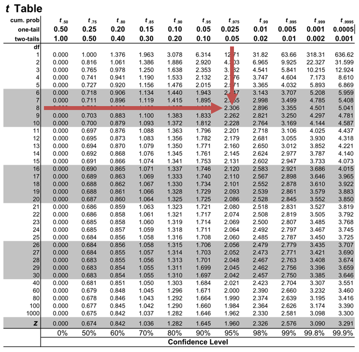
Notice that $|t|>t_{c}$ i.e., ($10.85>2.306$)

Therefore, we reject the null hypothesis and conclude that the estimated slope coefficient is statistically different from one.

Note that we used the confidence interval approach and arrived at the same conclusion.

Question Neeth Shinu, CFA, is forecasting price elasticity of supply for a certain product. Shinu uses the quantity of the product supplied for the past 5months as the dependent variable and the price per unit of the product as the independent variable. The regression results are shown below. $$\small{\begin{array}{lccccc}\hline \textbf{Regression Statistics} & & & & & \\ \hline \text{Multiple R} & 0.9971 & {}& {}&{}\\ \text{R Square} & 0.9941 & & & \\ \text{Adjusted R Square} & 0.9922 & & & & \\ \text{Standard Error} & 3.6515 & & & \\ \text{Observations} & 5 & & & \\ \hline {}& \textbf{Coefficients} & \textbf{Standard Error} & \textbf{t Stat} & \textbf{P-value}\\ \hline\text{Intercept} & -159 & 10.520 & (15.114) & 0.001\\ \text{Slope} & 0.26 & 0.012 & 22.517 & 0.000\\ \hline\end{array}}$$ Which of the following most likely reports the correct value of the t-statistic for the slope and most accurately evaluates its statistical significance with 95% confidence? A. $t=21.67$; slope is significantly different from zero. B. $t= 3.18$; slope is significantly different from zero. C. $t=22.57$; slope is not significantly different from zero. Solution The correct answer is A . The t-statistic is calculated using the formula: $$\text{t}=\frac{\widehat{b_{1}}-b_1}{\widehat{S_{b_{1}}}}$$ Where: $b_{1}$ = True slope coefficient $\widehat{b_{1}}$ = Point estimator for $b_{1}$ $\widehat{S_{b_{1}}}$ = Standard error of the regression coefficient $$\begin{align*}\text{t}&=\frac{0.26-0}{0.012}\\&=21.67\end{align*}$$ The critical two-tail t-values from the t-table with $n-2 = 3$ degrees of freedom are: $$t_{c}=±3.18$$ Notice that $|t|>t_{c}$ (i.e $21.67>3.18$). Therefore, the null hypothesis can be rejected. Further, we can conclude that the estimated slope coefficient is statistically different from zero.

Offered by AnalystPrep

Analysis of Variance (ANOVA)

Predicted value of a dependent variable, present values, future values, annuiti ....

Future Values The Future Value (FV) of a Single Sum of Cash Flow... Read More

Updating Probability Using Bayes’ Fo ...

Bayes’ formula is used to calculate an updated or posterior probability given a... Read More

Kurtosis refers to the measurement of the degree to which a given distribution... Read More

Monte-Carlo Simulation

Monte Carlo simulations are about producing many random variables based on specific probability... Read More

school Campus Bookshelves
menu_book Bookshelves
perm_media Learning Objects
login Login
how_to_reg Request Instructor Account
hub Instructor Commons
Download Page (PDF)
Download Full Book (PDF)
Periodic Table
Physics Constants
Scientific Calculator
Reference & Cite
Tools expand_more
Readability

selected template will load here

This action is not available.

12.5: Testing the Significance of the Correlation Coefficient

Last updated
Save as PDF
Page ID 800

The correlation coefficient, $r$, tells us about the strength and direction of the linear relationship between $x$ and $y$. However, the reliability of the linear model also depends on how many observed data points are in the sample. We need to look at both the value of the correlation coefficient $r$ and the sample size $n$, together. We perform a hypothesis test of the "significance of the correlation coefficient" to decide whether the linear relationship in the sample data is strong enough to use to model the relationship in the population.

The sample data are used to compute $r$, the correlation coefficient for the sample. If we had data for the entire population, we could find the population correlation coefficient. But because we have only sample data, we cannot calculate the population correlation coefficient. The sample correlation coefficient, $r$, is our estimate of the unknown population correlation coefficient.

The symbol for the population correlation coefficient is $\rho$, the Greek letter "rho."
$\rho =$ population correlation coefficient (unknown)
$r =$ sample correlation coefficient (known; calculated from sample data)

The hypothesis test lets us decide whether the value of the population correlation coefficient $\rho$ is "close to zero" or "significantly different from zero". We decide this based on the sample correlation coefficient $r$ and the sample size $n$.

If the test concludes that the correlation coefficient is significantly different from zero, we say that the correlation coefficient is "significant."

Conclusion: There is sufficient evidence to conclude that there is a significant linear relationship between $x$ and $y$ because the correlation coefficient is significantly different from zero.
What the conclusion means: There is a significant linear relationship between $x$ and $y$. We can use the regression line to model the linear relationship between $x$ and $y$ in the population.

If the test concludes that the correlation coefficient is not significantly different from zero (it is close to zero), we say that correlation coefficient is "not significant".

Conclusion: "There is insufficient evidence to conclude that there is a significant linear relationship between $x$ and $y$ because the correlation coefficient is not significantly different from zero."
What the conclusion means: There is not a significant linear relationship between $x$ and $y$. Therefore, we CANNOT use the regression line to model a linear relationship between $x$ and $y$ in the population.
If $r$ is significant and the scatter plot shows a linear trend, the line can be used to predict the value of $y$ for values of $x$ that are within the domain of observed $x$ values.
If $r$ is not significant OR if the scatter plot does not show a linear trend, the line should not be used for prediction.
If $r$ is significant and if the scatter plot shows a linear trend, the line may NOT be appropriate or reliable for prediction OUTSIDE the domain of observed $x$ values in the data.

PERFORMING THE HYPOTHESIS TEST

Null Hypothesis: $H_{0}: \rho = 0$
Alternate Hypothesis: $H_{a}: \rho \neq 0$

WHAT THE HYPOTHESES MEAN IN WORDS:

Null Hypothesis $H_{0}$ : The population correlation coefficient IS NOT significantly different from zero. There IS NOT a significant linear relationship(correlation) between $x$ and $y$ in the population.
Alternate Hypothesis $H_{a}$ : The population correlation coefficient IS significantly DIFFERENT FROM zero. There IS A SIGNIFICANT LINEAR RELATIONSHIP (correlation) between $x$ and $y$ in the population.

DRAWING A CONCLUSION:There are two methods of making the decision. The two methods are equivalent and give the same result.

Method 1: Using the $p\text{-value}$
Method 2: Using a table of critical values

In this chapter of this textbook, we will always use a significance level of 5%, $\alpha = 0.05$

Using the $p\text{-value}$ method, you could choose any appropriate significance level you want; you are not limited to using $\alpha = 0.05$. But the table of critical values provided in this textbook assumes that we are using a significance level of 5%, $\alpha = 0.05$. (If we wanted to use a different significance level than 5% with the critical value method, we would need different tables of critical values that are not provided in this textbook.)

METHOD 1: Using a $p\text{-value}$ to make a decision

Using the ti83, 83+, 84, 84+ calculator.

To calculate the $p\text{-value}$ using LinRegTTEST:

On the LinRegTTEST input screen, on the line prompt for $\beta$ or $\rho$, highlight "$\neq 0$"

The output screen shows the $p\text{-value}$ on the line that reads "$p =$".

(Most computer statistical software can calculate the $p\text{-value}$.)

If the $p\text{-value}$ is less than the significance level ( $\alpha = 0.05$ ):

Decision: Reject the null hypothesis.
Conclusion: "There is sufficient evidence to conclude that there is a significant linear relationship between $x$ and $y$ because the correlation coefficient is significantly different from zero."

If the $p\text{-value}$ is NOT less than the significance level ( $\alpha = 0.05$ )

Decision: DO NOT REJECT the null hypothesis.
Conclusion: "There is insufficient evidence to conclude that there is a significant linear relationship between $x$ and $y$ because the correlation coefficient is NOT significantly different from zero."

Calculation Notes:

You will use technology to calculate the $p\text{-value}$. The following describes the calculations to compute the test statistics and the $p\text{-value}$:
The $p\text{-value}$ is calculated using a $t$-distribution with $n - 2$ degrees of freedom.
The formula for the test statistic is $t = \frac{r\sqrt{n-2}}{\sqrt{1-r^{2}}}$. The value of the test statistic, $t$, is shown in the computer or calculator output along with the $p\text{-value}$. The test statistic $t$ has the same sign as the correlation coefficient $r$.
The $p\text{-value}$ is the combined area in both tails.

An alternative way to calculate the $p\text{-value}$ ( $p$ ) given by LinRegTTest is the command 2*tcdf(abs(t),10^99, n-2) in 2nd DISTR.

THIRD-EXAM vs FINAL-EXAM EXAMPLE: $p\text{-value}$ method

Consider the third exam/final exam example.
The line of best fit is: $\hat{y} = -173.51 + 4.83x$ with $r = 0.6631$ and there are $n = 11$ data points.
Can the regression line be used for prediction? Given a third exam score ( $x$ value), can we use the line to predict the final exam score (predicted $y$ value)?
$H_{0}: \rho = 0$
$H_{a}: \rho \neq 0$
$\alpha = 0.05$
The $p\text{-value}$ is 0.026 (from LinRegTTest on your calculator or from computer software).
The $p\text{-value}$, 0.026, is less than the significance level of $\alpha = 0.05$.
Decision: Reject the Null Hypothesis $H_{0}$
Conclusion: There is sufficient evidence to conclude that there is a significant linear relationship between the third exam score ($x$) and the final exam score ($y$) because the correlation coefficient is significantly different from zero.

Because $r$ is significant and the scatter plot shows a linear trend, the regression line can be used to predict final exam scores.

METHOD 2: Using a table of Critical Values to make a decision

The 95% Critical Values of the Sample Correlation Coefficient Table can be used to give you a good idea of whether the computed value of $r$ is significant or not . Compare $r$ to the appropriate critical value in the table. If $r$ is not between the positive and negative critical values, then the correlation coefficient is significant. If $r$ is significant, then you may want to use the line for prediction.

Example $\PageIndex{1}$

Suppose you computed $r = 0.801$ using $n = 10$ data points. $df = n - 2 = 10 - 2 = 8$. The critical values associated with $df = 8$ are $-0.632$ and $+0.632$. If $r <$ negative critical value or $r >$ positive critical value, then $r$ is significant. Since $r = 0.801$ and $0.801 > 0.632$, $r$ is significant and the line may be used for prediction. If you view this example on a number line, it will help you.

Exercise $\PageIndex{1}$

For a given line of best fit, you computed that $r = 0.6501$ using $n = 12$ data points and the critical value is 0.576. Can the line be used for prediction? Why or why not?

If the scatter plot looks linear then, yes, the line can be used for prediction, because $r >$ the positive critical value.

Example $\PageIndex{2}$

Suppose you computed $r = –0.624$ with 14 data points. $df = 14 – 2 = 12$. The critical values are $-0.532$ and $0.532$. Since $-0.624 < -0.532$, $r$ is significant and the line can be used for prediction

Horizontal number line with values of -0.624, -0.532, and 0.532.

Exercise $\PageIndex{2}$

For a given line of best fit, you compute that $r = 0.5204$ using $n = 9$ data points, and the critical value is $0.666$. Can the line be used for prediction? Why or why not?

No, the line cannot be used for prediction, because $r <$ the positive critical value.

Example $\PageIndex{3}$

Suppose you computed $r = 0.776$ and $n = 6$. $df = 6 - 2 = 4$. The critical values are $-0.811$ and $0.811$. Since $-0.811 < 0.776 < 0.811$, $r$ is not significant, and the line should not be used for prediction.

Horizontal number line with values -0.924, -0.532, and 0.532.

Exercise $\PageIndex{3}$

For a given line of best fit, you compute that $r = -0.7204$ using $n = 8$ data points, and the critical value is $= 0.707$. Can the line be used for prediction? Why or why not?

Yes, the line can be used for prediction, because $r <$ the negative critical value.

THIRD-EXAM vs FINAL-EXAM EXAMPLE: critical value method

Consider the third exam/final exam example. The line of best fit is: $\hat{y} = -173.51 + 4.83x$ with $r = 0.6631$ and there are $n = 11$ data points. Can the regression line be used for prediction? Given a third-exam score ( $x$ value), can we use the line to predict the final exam score (predicted $y$ value)?

Use the "95% Critical Value" table for $r$ with $df = n - 2 = 11 - 2 = 9$.
The critical values are $-0.602$ and $+0.602$
Since $0.6631 > 0.602$, $r$ is significant.
Conclusion:There is sufficient evidence to conclude that there is a significant linear relationship between the third exam score ($x$) and the final exam score ($y$) because the correlation coefficient is significantly different from zero.

Example $\PageIndex{4}$

Suppose you computed the following correlation coefficients. Using the table at the end of the chapter, determine if $r$ is significant and the line of best fit associated with each r can be used to predict a $y$ value. If it helps, draw a number line.

$r = –0.567$ and the sample size, $n$, is $19$. The $df = n - 2 = 17$. The critical value is $-0.456$. $-0.567 < -0.456$ so $r$ is significant.
$r = 0.708$ and the sample size, $n$, is $9$. The $df = n - 2 = 7$. The critical value is $0.666$. $0.708 > 0.666$ so $r$ is significant.
$r = 0.134$ and the sample size, $n$, is $14$. The $df = 14 - 2 = 12$. The critical value is $0.532$. $0.134$ is between $-0.532$ and $0.532$ so $r$ is not significant.
$r = 0$ and the sample size, $n$, is five. No matter what the $dfs$ are, $r = 0$ is between the two critical values so $r$ is not significant.

Exercise $\PageIndex{4}$

For a given line of best fit, you compute that $r = 0$ using $n = 100$ data points. Can the line be used for prediction? Why or why not?

No, the line cannot be used for prediction no matter what the sample size is.

Assumptions in Testing the Significance of the Correlation Coefficient

Testing the significance of the correlation coefficient requires that certain assumptions about the data are satisfied. The premise of this test is that the data are a sample of observed points taken from a larger population. We have not examined the entire population because it is not possible or feasible to do so. We are examining the sample to draw a conclusion about whether the linear relationship that we see between $x$ and $y$ in the sample data provides strong enough evidence so that we can conclude that there is a linear relationship between $x$ and $y$ in the population.

The regression line equation that we calculate from the sample data gives the best-fit line for our particular sample. We want to use this best-fit line for the sample as an estimate of the best-fit line for the population. Examining the scatter plot and testing the significance of the correlation coefficient helps us determine if it is appropriate to do this.

The assumptions underlying the test of significance are:

There is a linear relationship in the population that models the average value of $y$ for varying values of $x$. In other words, the expected value of $y$ for each particular value lies on a straight line in the population. (We do not know the equation for the line for the population. Our regression line from the sample is our best estimate of this line in the population.)
The $y$ values for any particular $x$ value are normally distributed about the line. This implies that there are more $y$ values scattered closer to the line than are scattered farther away. Assumption (1) implies that these normal distributions are centered on the line: the means of these normal distributions of $y$ values lie on the line.
The standard deviations of the population $y$ values about the line are equal for each value of $x$. In other words, each of these normal distributions of $y$ values has the same shape and spread about the line.
The residual errors are mutually independent (no pattern).
The data are produced from a well-designed, random sample or randomized experiment.

Linear regression is a procedure for fitting a straight line of the form $\hat{y} = a + bx$ to data. The conditions for regression are:

Linear In the population, there is a linear relationship that models the average value of $y$ for different values of $x$.
Independent The residuals are assumed to be independent.
Normal The $y$ values are distributed normally for any value of $x$.
Equal variance The standard deviation of the $y$ values is equal for each $x$ value.
Random The data are produced from a well-designed random sample or randomized experiment.

The slope $b$ and intercept $a$ of the least-squares line estimate the slope $\beta$ and intercept $\alpha$ of the population (true) regression line. To estimate the population standard deviation of $y$, $\sigma$, use the standard deviation of the residuals, $s$. $s = \sqrt{\frac{SEE}{n-2}}$. The variable $\rho$ (rho) is the population correlation coefficient. To test the null hypothesis $H_{0}: \rho =$ hypothesized value , use a linear regression t-test. The most common null hypothesis is $H_{0}: \rho = 0$ which indicates there is no linear relationship between $x$ and $y$ in the population. The TI-83, 83+, 84, 84+ calculator function LinRegTTest can perform this test (STATS TESTS LinRegTTest).

Formula Review

Least Squares Line or Line of Best Fit:

\[\hat{y} = a + bx\]

\[a = y\text{-intercept}\]

\[b = \text{slope}\]

Standard deviation of the residuals:

\[s = \sqrt{\frac{SSE}{n-2}}\]

\[SSE = \text{sum of squared errors}\]

\[n = \text{the number of data points}\]

IMAGES

PPT
Correlation vs Regression
Correlation and Regression Analysis: Learn Everything With Examples
Correlation Coefficient Formula
PPT
Correlation and Regression

VIDEO

Hypothesis Testing in Simple Linear Regression
Inferences for Regression & Correlation
Correlation and Regression in Research methodology
Correlation vs Regression: What's the difference?
Hypothesis Testing based on Correlation
Correlation Hypothesis Test Theory

COMMENTS

12.2.1: Hypothesis Test for Linear Regression
The test statistic value is the same value of the t-test for correlation even though they used different formulas. We look in the same place using technology as the correlation test. The test statistic is greater than the critical value of 2.160 and in the rejection region. The decision is to reject $H_{0}$.
11.2: Correlation Hypothesis Test
The p-value is calculated using a t -distribution with n − 2 degrees of freedom. The formula for the test statistic is t = r√n − 2 √1 − r2. The value of the test statistic, t, is shown in the computer or calculator output along with the p-value. The test statistic t has the same sign as the correlation coefficient r.
12.1.2: Hypothesis Test for a Correlation
The t-test is a statistical test for the correlation coefficient. It can be used when x x and y y are linearly related, the variables are random variables, and when the population of the variable y y is normally distributed. The formula for the t-test statistic is t = r ( n − 2 1 −r2)− −−−−−−−√ t = r ( n − 2 1 − r 2).
12.4 Testing the Significance of the Correlation Coefficient
The correlation coefficient, r, tells us about the strength and direction of the linear relationship between x and y.However, the reliability of the linear model also depends on how many observed data points are in the sample. We need to look at both the value of the correlation coefficient r and the sample size n, together.. We perform a hypothesis test of the "significance of the correlation ...
1.9
Let's perform the hypothesis test on the husband's age and wife's age data in which the sample correlation based on n = 170 couples is r = 0.939. To test H 0: ρ = 0 against the alternative H A: ρ ≠ 0, we obtain the following test statistic: t ∗ = r n − 2 1 − R 2 = 0.939 170 − 2 1 − 0.939 2 = 35.39. To obtain the P -value, we need ...
Hypothesis Test for Correlation
The hypothesis test lets us decide whether the value of the population correlation coefficient ρ is "close to zero" or "significantly different from zero.". We decide this based on the sample correlation coefficient r and the sample size n. If the test concludes that the correlation coefficient is significantly different from zero, we ...
Statistics review 7: Correlation and regression
The same assumptions are needed in testing the null hypothesis that the correlation is 0, but in order to interpret confidence intervals for the correlation coefficient both variables must be Normally distributed. Both correlation and regression assume that the relationship between the two variables is linear.
Hypothesis Testing: Correlations
We perform a hypothesis test of the "significance of the correlation coefficient" to decide whether the linear relationship in the sample data is strong enough to use to model the relationship in the population. The hypothesis test lets us decide whether the value of the population correlation coefficient. \rho ρ.
Interpreting Correlation Coefficients
Hypothesis Test for Correlation Coefficients. Correlation coefficients have a hypothesis test. As with any hypothesis test, this test takes sample data and evaluates two mutually exclusive statements about the population from which the sample was drawn. ... Instead of correlation, I'd use regression with an interaction effect. I'd want to ...
Correlation Coefficient
A correlation coefficient tells you the strength of the relationship between variables using a single number between -1 and 1. ... Hypothesis testing. Hypothesis testing guide; Null vs. alternative hypotheses; Statistical significance; ... A regression analysis helps you find the equation for the line of best fit, and you can use it to predict ...
Pearson Correlation Coefficient (r)
Revised on February 10, 2024. The Pearson correlation coefficient (r) is the most common way of measuring a linear correlation. It is a number between -1 and 1 that measures the strength and direction of the relationship between two variables. When one variable changes, the other variable changes in the same direction.
Correlation vs. Regression: What's the Difference?
Differences: Regression is able to show a cause-and-effect relationship between two variables. Correlation does not do this. Regression is able to use an equation to predict the value of one variable, based on the value of another variable. Correlation does not does this. Regression uses an equation to quantify the relationship between two ...
2.5.2 Hypothesis Testing for Correlation
It is also possible to use a hypothesis test to determine whether a given product moment correlation coefficient calculated from a sample could be representative of the same relationship existing within the whole population. For full information on hypothesis testing, see the revision notes from section 5.1.1 Hypothesis Testing
Understanding the Null Hypothesis for Linear Regression
x: The value of the predictor variable. Simple linear regression uses the following null and alternative hypotheses: H0: β1 = 0. HA: β1 ≠ 0. The null hypothesis states that the coefficient β1 is equal to zero. In other words, there is no statistically significant relationship between the predictor variable, x, and the response variable, y.
Regression, Correlation and Hypothesis Testing
Correlation:. All Correlation is Causation: Students often believe that if two variables are correlated, one must cause the other.; Strength of Correlation: Students might think a correlation coefficient of r=0.5 means one variable is "half caused" by the other.; Perfect Correlation: Some believe that a correlation coefficient of exactly 1 or -1 means the data points fall perfectly on a ...
Hypothesis Test for Regression and Correlation Analysis
In testing the hypothesis for regression and correlation can used two ways, namely: Hypothesis Test with P-Value. In testing the hypothesis, it can be seen from the p-value. In formulating a hypothesis, we need to determine an alpha value that we will use. Experimental studies generally use 5% and 1%.
How to Write a Hypothesis for Correlation
A hypothesis is a testable statement about how something works in the natural world. While some hypotheses predict a causal relationship between two variables, other hypotheses predict a correlation between them. According to the Research Methods Knowledge Base, a correlation is a single number that describes the relationship between two variables.
Hypothesis Testing in Regression Analysis
Reject the null hypothesis if the absolute value of the t-statistic is greater than the critical t-value i.e., $t\ >\ +\ t_{critical}\ or\ t\ <\ -t_{\text{critical}}$. Example: Hypothesis Testing of the Significance of Regression Coefficients. An analyst generates the following output from the regression analysis of inflation on unemployment:
3.3.4: Hypothesis Test for Simple Linear Regression
Simple Linear Regression ANOVA Hypothesis Test Example: Rainfall and sales of sunglasses We will now describe a hypothesis test to determine if the regression model is meaningful; in other words, does the value of $X$ in any way help predict the expected value of $Y$?
Six Sigma Correlation, Regression, and Hypothesis Testing
Study with Quizlet and memorize flashcards containing terms like The power of a hypothesis test is the likelihood that you will discover a significant difference in your process when one exists. What factors affect the power of a hypothesis test?, Why might a Six Sigma team determine the statistical significance of a correlation coefficient?, In what ways can you use correlation analysis in ...
Six Sigma Correlation, Regression, and Hypothesis Testing
Quiz yourself with questions and answers for Six Sigma Correlation, Regression, and Hypothesis Testing, so you can be ready for test day. Explore quizzes and practice tests created by teachers and students or create one from your course material.
6Sigma Correlation and Regression Flashcards
Strong correlation or regression between 2 variables does not indicate a causal relationship. This is a critical concept to understand, because attributing causation because correlation is strong can mean making poor decisions regarding a process. 2. This tool is usually deployed by 6sigma teams in the Measure, Analyze, or Improve phase of the ...
12.5: Testing the Significance of the Correlation Coefficient
The p-value is calculated using a t -distribution with n − 2 degrees of freedom. The formula for the test statistic is t = r√n − 2 √1 − r2. The value of the test statistic, t, is shown in the computer or calculator output along with the p-value. The test statistic t has the same sign as the correlation coefficient r.
PDF Homework # 12 (correlation and regression) Do NOT use R for problems 1
You should arrange this into a regression equation: Ŷ = 10.778 - 0.9537 X Note that the given p-value is .00999.If the test is one sided, then you need to do: 0.00999/2 = .004995 (in either case, the test would be significant at α = 0.01) Finally, notice that the R2 is 0.5845. If everything else is okay (e.g. residual plots), we can say

12.4 Testing the Significance of the Correlation Coefficient

PERFORMING THE HYPOTHESIS TEST

METHOD 1: Using a p -value to make a decision

METHOD 2: Using a table of Critical Values to make a decision

Example 12.7

Try It 12.7

Example 12.8

Try It 12.8

Example 12.9

Try It 12.9

THIRD-EXAM vs FINAL-EXAM EXAMPLE: critical value method

Example 12.10

Try It 12.10

Assumptions in Testing the Significance of the Correlation Coefficient

User Preferences

Keyboard Shortcuts

Steps for Hypothesis Testing for \(\boldsymbol{\rho}\) Section

Step 2: Test Statistic

Step 3: P-Value

Step 4: Decision

Example 1-5: Husband and Wife Data Section

Student's t distribution with 168 DF

Correlation: WAge, HAge

Final Note Section

Module 12: Linear Regression and Correlation

Performing the Hypothesis Test

What the Hypotheses Mean in Words

Drawing a Conclusion

Method 1: Using a p -value to make a decision

Recall: ORDER OF OPERATIONS

THIRD-EXAM vs FINAL-EXAM EXAM: p- value method

Method 2: Using a table of Critical Values to make a decision

THIRD-EXAM vs FINAL-EXAM EXAMPLE: critical value method

Assumptions in Testing the Significance of the Correlation Coefficient

Statistics review 7: Correlation and regression

Jonathan Ball

Introduction

Scatter diagram

Correlation

Hypothesis test of correlation

Confidence interval for the population correlation coefficient

Misuse of correlation

Equation of a straight line

Method of least squares

Hypothesis tests and confidence intervals

Analysis of variance

Coefficent of determination

Assumptions and limitations

Competing interests

Abbreviations

Understanding the Null Hypothesis for Linear Regression

Example 1: Simple Linear Regression

Example 2: Multiple Linear Regression

Additional Resources

Published by Zach

Regression, Correlation and Hypothesis Testing

Success Criteria

Key Concepts

Common Misconceptions

Mr Mathematics Blog

GCSE Trigonometry Skills & SOH CAH TOA Techniques

Regions in the Complex Plane

Hypothesis Test for Regression and Correlation Analysis

Understanding the Essence of the Difference Between Descriptive Statistics and Inferential Statistics in Research

Most Popular

How to Calculate a P-Value

Related Articles

Find Your Next Great Science Fair Project! GO

Hypothesis Testing in Regression Analysis

The t-test Approach

Example: Hypothesis Testing of the Significance of Regression Coefficients

Analysis of Variance (ANOVA)

Updating Probability Using Bayes’ Fo ...

Monte-Carlo Simulation

12.5: Testing the Significance of the Correlation Coefficient

PERFORMING THE HYPOTHESIS TEST

METHOD 1: Using a \(p\text{-value}\) to make a decision

METHOD 2: Using a table of Critical Values to make a decision

Example \(\PageIndex{1}\)

Exercise \(\PageIndex{1}\)